Apache Iceberg Observability: Monitoring & Metrics for Data Lake Tables

Introduction​

Modern data lakes can become a black box: pipelines break or slow down, and engineers scramble to find out why. Issues like a sudden schema change or a sudden increase of tiny files can lurk undetected until they impact production. Apache Iceberg tackles this challenge by making your data lake self-observing. Iceberg tables are self-describing, exposing a goldmine of operational metadata that is fully queryable and deeply insightful. Instead of blind spots, you get built-in visibility into the health, structure, and behavior of your data. For example, you can ask Iceberg via SQL:

• How many files does this table have?
• Which partitions have lots of small files?
• Did someone alter the schema recently?

And get answers immediately from the table’s metadata. Iceberg’s design effectively turns metadata into an observability layer for your data platform, enabling proactive data lake monitoring and allowing data engineers to shift from reactive firefighting to preventive operations.

-- How many data files does the table currently have?
SELECT COUNT(*) AS data_file_count
FROM prod.db.orders.files
WHERE content = 0;

-- Which partitions have many small files?
SELECT
  partition.order_date,
  COUNT(*) AS file_count,
  ROUND(AVG(file_size_in_bytes) / 1024 / 1024, 2) AS avg_file_size_mb
FROM prod.db.orders.files
WHERE content = 0
GROUP BY partition.order_date
HAVING AVG(file_size_in_bytes) < 64 * 1024 * 1024
ORDER BY file_count DESC;

In this blog, we’ll dive deep into how to leverage Apache Iceberg’s observability features. We’ll explore how to introspect table health using Iceberg’s metadata tables and demonstrate hands-on examples of querying these metadata. We’ll also discuss new metrics and alerting capabilities introduced in Iceberg, and how they enable real-time monitoring and automated maintenance. Along the way, we’ll compare Iceberg’s approach with other data lake table formats, to understand why Iceberg stands out for data observability. The audience is data engineers, so expect a technical deep dive with SQL examples and practical scenarios.

Monitoring Table Health Using Iceberg Metadata Tables​

Apache Iceberg observability centers on its queryable Iceberg metadata tables. These are like built-in system tables that describe your Iceberg table’s state and history. Unlike external logs or ad-hoc scripts, Iceberg’s metadata tables can be queried with standard SQL in your processing engine of choice. Think of them as Iceberg’s modern answer to legacy commands like SHOW PARTITIONS, but far more powerful and flexible. In traditional Hadoop or Hive setups, getting insight into file counts, schemas, or partitions often required engine-specific tools or painstaking manual steps. In Iceberg, all that information is available as structured tables that you can join, filter, and aggregate as needed. In short, the Iceberg table contains not just your data, but rich metadata about the data all accessible via SQL.

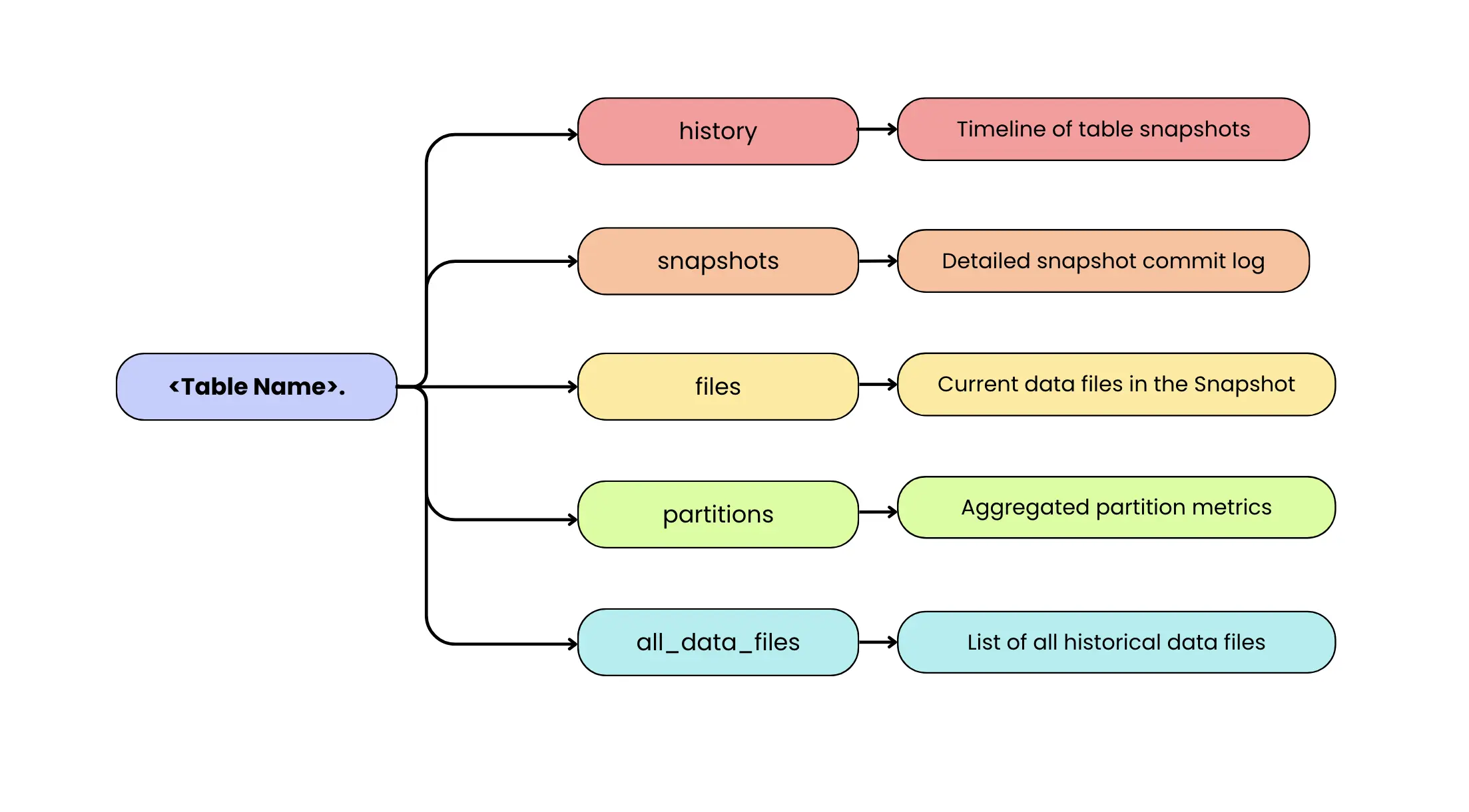
• <table_name>.history: A timeline of table snapshots (versions) and their timestamps, like a version control log of all changes. This shows when each snapshot was made current, helping track the evolution of the table over time (e.g. when data was updated or when the schema changed).

• <table_name>.snapshots: A detailed log of every snapshot of the table, with one row per snapshot. It includes metadata like the snapshot ID, parent snapshot ID (helps lineage), timestamp committed, and the operation (e.g. append, overwrite, delete) that produced that snapshot. It also contains a summary of changes (like number of records or files added/removed). This table makes it easy to audit how the table has evolved and identify what each commit did.

• <table_name>.files: It is the most direct “what’s in the table right now?” view in Iceberg. It lists all files that make up the current table state, including both data files (Parquet/ORC/Avro) and delete files (positional and equality deletes). Each row includes operational details such as the file path, format, partition values, record count, file size, and (when available) file-level column metrics. If you want to narrow the view to specific file classes, use the content column: content = 0 filters to data files, content = 1 to positional delete files, and content = 2 to equality delete files. In practice, you’ll query files when you want a unified view of everything the table will read, and use <table_name>.data_files or <table_name>.delete_files when you want only one category without applying filters.

• <table_name>.partitions: An aggregated view of how data is partitioned in the table. Each row represents a partition (or chunk of the data, e.g. a date or bucket) and includes metrics like the number of files in that partition, total records, total size in bytes, and even counts of deletes in that partition. It also records the partition’s last update time and snapshot ID. This is invaluable for spotting skew or imbalance – for example, if one partition has hundreds of tiny files while others have few, or if a partition hasn’t been updated in a long time (stale data).

• <table_name>.all_data_files: It is the historical counterpart to <table_name>.data_files. Instead of showing only the files in the current snapshot, it lists data files referenced across all snapshots that are still tracked by the table’s metadata. This makes it useful for longitudinal analysis like understanding how file counts and total data volume evolve over time, spotting churn from rewrites/compaction, or estimating storage overhead from retained history. Because it’s snapshot-aware, the same physical file can appear multiple times if it remained referenced across multiple snapshots. Also note that this isn’t an eternal record: once you expire snapshots and clean up metadata, older snapshots (and the files only referenced by them) may stop appearing in all_data_files, since the table no longer tracks that historical state.

There are a few other metadata tables as well, like manifests, all_manifests, metadata_log_entries, etc., but the ones above are the most directly useful for monitoring table health. metadata_log_entries logs every metadata file change (table schema or config update) and can help track changes in table definition. manifests tables show how data files are grouped into manifest files, which can help debug performance issues at the manifest level, though that’s a more advanced use case.

With these metadata tables, Iceberg lets you ask a variety of health-check questions via SQL. Below we walk through several important monitoring aspects and how to address them using Iceberg metadata.

Tracking Data File Counts and Sizes (Small Files Problem)​

One of the most common issues in data lakes is the small files problem: highly parallel or streaming writers generate many tiny files, increasing query planning overhead and degrading read performance. In a truly observable system, this problem should be detected automatically, not by someone periodically inspecting the table.

When metrics reporting is enabled, Iceberg can emit commit- and scan-level reports (CommitReport / ScanReport) during writes and reads. You can forward these events into your monitoring stack and evaluate file-size patterns (like “average file size dropping below X”) over a window of multiple commits to avoid alert noise from one-off small batches. In this setup, metrics provide the always-on detection signal, while Iceberg’s metadata tables (files, partitions, snapshots) remain the fastest way to diagnose the root cause once an alert fires.

Iceberg’s metadata tables still play a critical supporting role. After an alert is raised, engineers can query metadata tables such as table.files or table.partitions to investigate why the average file size dropped whether it was caused by a specific partition, a misconfigured writer, or a sudden change in ingestion patterns. In this sense, continuous metrics detect the problem, and metadata queries explain it.

SELECT
  partition.order_date AS order_date,
  COUNT(*) AS data_file_count,
  ROUND(AVG(file_size_in_bytes) / 1024 / 1024, 2) AS avg_data_file_size_mb
FROM prod.db.orders.files
WHERE content = 0                       -- DATA files
GROUP BY partition.order_date
HAVING AVG(file_size_in_bytes) < 64 * 1024 * 1024
ORDER BY data_file_count DESC;

This query surfaces partitions that are likely suffering from the small-files problem. It groups data files by partition (order_date), counts how many data files exist per partition, and computes the average file size for each group. By filtering on partitions where the average file size falls below 64 MB, it highlights partitions where data is fragmented into many small files. The result makes it easy to see which partitions are problematic (high file count, low average size) and therefore prime candidates for compaction or rewrite operations.

By separating detection (metrics) from diagnosis (SQL), Iceberg enables proactive, production-grade monitoring of small files while retaining deep introspection capabilities when needed.

Monitoring Table Growth, Trends, and Capacity Planning​

Beyond detecting sudden anomalies, continuous Iceberg metrics are equally critical for capacity planning and long-term trend analysis.

Because Iceberg emits commit-level metrics on every write, teams can track how a table evolves over time by accumulating snapshot changes. Metrics such as records added and bytes written naturally form a time series that represents a table’s growth trajectory.

Using Spark SQL, this data can be aggregated directly from the snapshots metadata table:

SELECT
  to_date(committed_at) AS commit_date,
  SUM(CAST(summary['added-records'] AS BIGINT)) AS records_added,
  ROUND(
    SUM(CAST(summary['added-files-size'] AS BIGINT)) / 1024 / 1024 / 1024,
    2
  ) AS gb_added
FROM prod.db.orders.snapshots
GROUP BY to_date(committed_at)
ORDER BY commit_date;

This enables engineers to:

• plot table growth over time
• track row count increases per day or week
• forecast future storage requirements
• validate whether growth aligns with expected business patterns

A slow, steady increase in records may be normal, while a sudden surge in bytes or row counts typically signals a meaningful shift in upstream behavior. Sometimes that shift is expected (for example, a seasonal traffic spike, a product launch, or a legitimate one-time historical load). Other times, it can indicate an ingestion issue like an accidentally re-triggered backfill that starts replaying large historical ranges (runaway backfill), a duplicate load, or a misconfigured job writing more data than intended. Conversely, an unexpected drop in records or bytes written can point to unintended deletes/overwrites, filters being applied incorrectly upstream, or a pipeline that silently stopped emitting a subset of data.

In practice, these queries are often run on a schedule and fed into dashboards or alerting systems, turning Iceberg’s metadata into continuous, time-series observability signals rather than ad-hoc inspections.

Explaining anomalies with Iceberg metadata​

When such alerts fire, Iceberg’s metadata provides the necessary context to explain why the change occurred. Each snapshot records not just what changed, but how it changed.

SELECT
  committed_at,
  operation,
  CAST(summary['added-records'] AS BIGINT) AS records_added,
  CAST(summary['added-files-size'] AS BIGINT) / (1024.0*1024*1024) AS gb_added
FROM prod.db.orders.snapshots
ORDER BY committed_at DESC
LIMIT 5;

From this, engineers can correlate anomalies with:

• commit timestamps
• operation types (append, overwrite, delete, compaction)
• records and data volume added or removed
• snapshot authors or application identifiers (when configured)

This makes it straightforward to determine whether a spike was caused by a planned backfill, a compaction job, or an unexpected write without digging through external logs or pipeline code.

In practice, this creates a clean separation of responsibilities:

• Metrics surface trends and anomalies early
• Metadata explains root causes during investigation

Together, they support both short-term alerting and long-term capacity forecasting.

Total Data (tracked history) vs Active Data​

Crucially, Iceberg’s metadata also tracks data that is no longer active. If you retain older snapshots for time travel or auditing, those files continue to consume storage even though they are not part of the latest table state. By comparing the files and all_data_files metadata tables, teams can quantify this overhead directly:

WITH active AS (
  SELECT SUM(file_size_in_bytes) AS bytes
  FROM prod.db.orders.files
  WHERE content = 0                 -- only DATA files
),
historical AS (
  SELECT SUM(file_size_in_bytes) AS bytes
  FROM prod.db.orders.all_data_files
)
SELECT
  ROUND(active.bytes / 1024 / 1024 / 1024, 2) AS active_data_gb,
  ROUND(historical.bytes / 1024 / 1024 / 1024, 2) AS total_data_gb,
  ROUND(historical.bytes / active.bytes, 2) AS data_bloat_ratio
FROM active, historical;

If total storage is significantly larger than active storage (for example, 5× or more), it indicates excessive snapshot or time-travel overhead. This is a strong signal to review retention policies or run snapshot cleanup explicitly:

spark.sql("""
  CALL prod.system.expire_snapshots(
    table => 'prod.db.orders',
    older_than => TIMESTAMP '2025-03-01',
    retain_last => 5
  )
""")

This procedure removes snapshot references older than March 1, 2025 (so the table stops tracking those historical versions) while keeping the latest 5 snapshots for safety and recent time travel. After expiring snapshots, a separate cleanup step (e.g., remove_orphan_files in many environments) is typically used to delete unreferenced data files from storage, depending on your catalog/runtime setup.

Snapshots accumulate until they’re expired by a maintenance operation like expireSnapshots / CALL … expire_snapshots. Many teams run this on a schedule; some platforms may automate it, but it’s not automatic by default in core Iceberg. Cloud providers such as AWS even recommend tracking a metric like Total Storage vs. Active Storage to make this overhead visible. Monitoring it regularly helps prevent silent storage bloat and avoids unnecessary cost.

Detecting Schema and Partition Changes​

Undocumented schema and partition changes are one of the most common causes of downstream data failures. A new column added without coordination, a renamed field, or a modified partition spec can silently break ETL jobs, dashboards, and ML pipelines. Apache Iceberg mitigates this risk by treating schema and partition evolution as first-class, versioned metadata, and Spark SQL provides a natural way to audit and validate these changes.

Every time an Iceberg table’s schema or partition spec is modified, Iceberg writes a new metadata version and records the change as a snapshot or metadata update. Importantly, these changes are visible even when no data files are added or removed, making them easy to miss in traditional data lakes but explicit in Iceberg.

Detecting schema-only changes using Spark SQL​

In Iceberg, these changes are recorded as new table metadata versions (new metadata.json files). Importantly, snapshots represent changes to data state, so a schema/spec change can occur without creating a new snapshot. That’s why the most reliable place to detect structural change is the metadata log, not the snapshots table

Detect schema evolution via metadata_log_entries (Spark SQL)​

In Spark, metadata_log_entries provides a chronological log of table metadata files along with the latest schema ID for each metadata version.

WITH log AS (
  SELECT
    timestamp,
    latest_snapshot_id,
    latest_schema_id,
    latest_sequence_number,
    LAG(latest_schema_id) OVER (
      ORDER BY timestamp, latest_sequence_number
    ) AS prev_schema_id,
    file AS metadata_file
  FROM prod.db.orders.metadata_log_entries
)
SELECT
  timestamp,
  latest_snapshot_id,
  prev_schema_id,
  latest_schema_id AS new_schema_id,
  metadata_file
FROM log
WHERE prev_schema_id IS NOT NULL
  AND latest_schema_id IS NOT NULL
  AND latest_schema_id <> prev_schema_id
ORDER BY timestamp DESC, latest_sequence_number DESC;

How to interpret the output:

• prev_schema_id: new_schema_id changing means a schema update happened.
• latest_snapshot_id tells you what data snapshot was current at that metadata version:
  • If latest_snapshot_id also changes around the same time, the schema change likely happened alongside a data commit.
  • If latest_snapshot_id stays the same, it was likely a metadata-only schema update (no new snapshot).

Validating schema changes across snapshots​

Spark time travel by snapshot ID / timestamp uses the snapshot’s schema (for VERSION AS OF <snapshot-id> / TIMESTAMP AS OF <ts>), which is perfect when the schema change is associated with a new snapshot boundary.

-- show recent snapshots
SELECT snapshot_id, committed_at, operation
FROM prod.db.orders.snapshots
ORDER BY committed_at DESC
LIMIT 10;

-- time travel by snapshot id (Spark + Iceberg)
SELECT * FROM prod.db.orders VERSION AS OF 10963874102873 LIMIT 0;

-- time travel by timestamp
SELECT * FROM prod.db.orders TIMESTAMP AS OF '2025-03-01 00:00:00' LIMIT 0;

However, if the schema change was metadata-only (no new snapshot), there may not be a “before” snapshot to time travel to, because the table’s current snapshot did not change. In that case, metadata_log_entries.metadata_file gives you the exact metadata JSON file to inspect/parse with Iceberg tooling (this is the authoritative record of the schema/spec at that point in time).

Practical monitoring pattern​

A production-friendly approach is to build a “schema evolution timeline” directly from metadata_log_entries:

• alert when latest_schema_id changes outside approved windows
• include metadata_file in the alert payload so an on-call engineer can inspect the exact metadata version
• (optionally) correlate with snapshots using latest_snapshot_id to see whether it coincided with a write

This keeps detection accurate even when schema changes don’t create snapshots.

Monitoring partition evolution​

Partition changes are just as critical as schema changes. A modified partition spec can alter data layout, query performance, and cost characteristics. Since Iceberg records partition metadata explicitly, Spark SQL can be used to monitor these changes as well.

For example, engineers can track shifts in partition structure or distribution by inspecting the partitions metadata table over time. A sudden increase in partition count or the appearance of unexpected partition values can signal that partitioning logic has changed upstream.

In practice, many teams combine these Spark SQL checks with lightweight governance rules:

• alert on schema changes outside approved deployment windows
• require review for partition-spec updates
• maintain a schema evolution timeline for auditability

By making schema and partition evolution fully observable and queryable, Iceberg eliminates “silent” structural changes. Spark SQL turns that metadata into an actionable audit layer, allowing teams to catch breaking changes early, validate them confidently, and keep their data platform stable as it evolves.

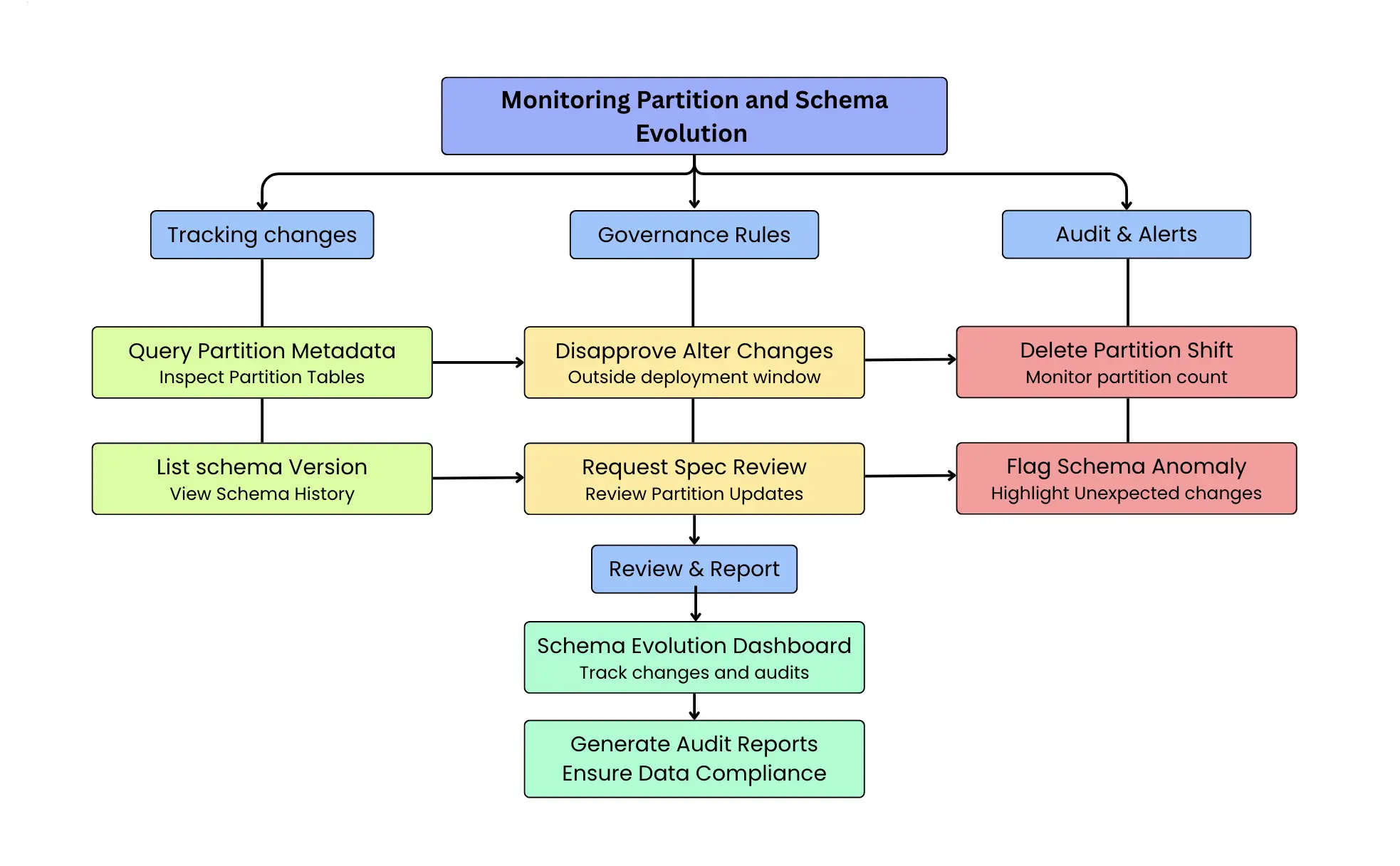
One practical approach is to set up a “schema evolution dashboard” that tracks when schema changes were introduced and by whom. Using Iceberg’s history, you could list out all schema versions over time. If your organization has a governance process for schema changes, this provides a cross-check any change not accounted for in the process can be flagged immediately. All of this is achieved without any external tracking mechanism, purely by leveraging Iceberg’s native metadata.

Hands-On Example: Observing a Table’s Lifecycle​

To make the observability concepts concrete, consider an Iceberg table orders, partitioned by order_date, and walk through a typical sequence of operations and the metadata Iceberg records at each step.

Initial insert​

After an initial batch insert, Iceberg creates a new snapshot with an append operation. The orders.files metadata table lists the newly added data files, including their file sizes and partition values. For example, after inserting a batch of data, the table may contain several data files of roughly similar size (e.g: ~64 MB each, depending on writer configuration).

The corresponding entry in orders.snapshots includes:

• The snapshot ID
• The commit timestamp
• The operation type (append)
• Summary metrics such as the number of records and files added

At the same time, orders.partitions reflects which partitions were affected and exposes per-partition statistics like file_count and record_count.

Updates and deletes​

When updates or deletes are performed, Iceberg’s metadata reflects the chosen write mode, and this directly influences what engineers need to monitor.

In copy-on-write (COW) mode, updates and deletes are applied by rewriting data files. No delete files are produced in this mode only data files exist. Each operation results in new data files that replace the old ones, and the corresponding snapshot records the operation type (append, delete, or overwrite) along with summary statistics such as the number of rows and files affected. As a result, observability in COW primarily focuses on the data-file layout: a growing number of small data files increases planning overhead and read amplification, making compaction or rewrite operations necessary.

In merge-on-read (MOR) mode, updates and deletes are represented using delete files in addition to data files. These delete files are tracked alongside data files in the orders.files metadata table and can be distinguished using the content column. Snapshot entries again record the operation type and summary metrics, but engineers must monitor two dimensions: (a) the accumulation of delete files, which increases merge work during reads, and (b) the underlying data-file layout, where small data files still negatively impact planning efficiency. A sustained rise in either delete files or small data files is a strong signal that compaction or rewrite maintenance should be triggered.

Detecting anomalous writes​

If a duplicate load occurs for example, an insert job is accidentally re-run the resulting snapshot will show an unusual increase in added files or records. This is immediately visible in the orders.snapshots table by inspecting the snapshot summaries.

Because Iceberg preserves snapshot history, engineers can identify the exact snapshot where the anomaly occurred and use time travel to inspect the table state before the problematic commit. The orders.history table provides the snapshot lineage required to safely roll back to a known-good snapshot if needed.

Debugging pipeline failures​

Throughout this lifecycle, Iceberg’s metadata eliminates the need for manual storage inspection or custom logging. For example, if a downstream job fails, engineers can inspect the most recent table activity with:

SELECT *
FROM prod.db.orders.snapshots
ORDER BY committed_at DESC
LIMIT 1;

This immediately reveals the last operation performed such as an unexpected schema change or delete which often explains downstream breakages. This tight feedback loop significantly reduces debugging time and makes table behavior transparent throughout its lifecycle.

Proactive Monitoring with Dashboards, Alerts, and Metrics Reporters​

Iceberg’s metadata is not only useful for ad-hoc inspection and debugging. It can also be used to build continuous observability pipelines that monitor table health, detect anomalies early, and trigger automated maintenance. In practice, teams capture Iceberg metrics using two complementary mechanisms: scheduled metadata queries and runtime metrics reporters.

Scheduled metadata queries (pull-based monitoring)​

The most common approach is to periodically query Iceberg’s metadata tables and materialize the results into a monitoring system. Because metadata tables are transactional and immutable, they are safe to query continuously and provide a reliable historical record of table behavior.

For example, the following Spark SQL job aggregates commit-level growth metrics over time:

val growthMetrics =
  spark.sql("""
    SELECT
      date_trunc('hour', committed_at) AS window_start,
      COUNT(*) AS commits,
      SUM(CAST(summary['added-records'] AS BIGINT)) AS records_added,
      SUM(CAST(summary['added-files-size'] AS BIGINT)) AS bytes_added
    FROM prod.db.orders.snapshots
    WHERE committed_at >= current_timestamp() - INTERVAL 1 DAY
    GROUP BY date_trunc('hour', committed_at)
  """)

growthMetrics.writeTo("prod.metrics.orders_growth").append()

This produces a durable time-series view of table growth that can be plotted in dashboards or evaluated by alerting rules. Sudden spikes in records or bytes written stand out immediately, enabling teams to detect backfills, misconfigured jobs, or duplicate ingestion early.

Because this approach is pull-based, it works with any Iceberg catalog and requires no changes to ingestion pipelines. It is especially effective for trend analysis, capacity planning, and SLA monitoring.

Alerting and anomaly detection using metadata​

Once metrics are materialized, alerting logic becomes straightforward. Teams typically compare recent behavior against historical baselines to detect abnormal growth or unexpected deletions.

For example, a simple check might flag a write surge when today’s record volume exceeds the recent daily average by a large factor:

if (todayRecords > historicalAverage * 3) {
  // trigger alert
}

When an alert fires, the next step is fast triage: jump to the most recent entries in table.snapshots (using the snapshot inspection query shown earlier) to confirm what changed and whether it was an expected event (e.g., planned backfill/compaction) or an unintended write pattern. This keeps the flow clean: metrics raise the alarm; metadata pinpoints the “what changed” quickly.

Runtime metrics with Iceberg metrics reporters (push-based monitoring)​

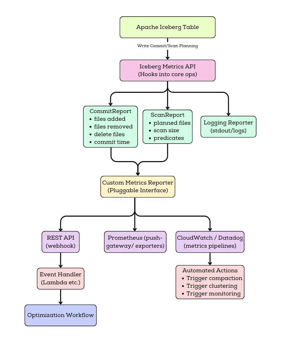
For near-real-time observability, Iceberg supports a pluggable Metrics Reporting framework (available since Iceberg 1.1.0) that emits CommitReport and ScanReport events which can be forwarded to your monitoring stack. Metrics reporters emit statistics automatically during table scans and commits, without requiring scheduled queries.

When enabled, Iceberg produces metrics such as:

• Number and size of files added or removed per commit
• Commit duration and retry counts
• Scan planning statistics and filter effectiveness

In Spark, a metrics reporter can be enabled via catalog configuration, enable a reporter via catalog config (e.g., LoggingMetricsReporter for validation or a custom reporter to Prometheus/OTel/etc.):

# Catalog-level metrics reporter (fully-qualified class name)

spark.sql.catalog.prod.metrics-reporter-impl=org.apache.iceberg.metrics.LoggingMetricsReporter

If you are using RESTCatalog, Iceberg uses RESTMetricsReporter by default with RESTCatalog, and you can toggle sending metrics like this:

# Toggle REST metrics reporting for a RESTCatalog:
spark.sql.catalog.prod.rest-metrics-reporting-enabled=true   # enable sending metrics
# spark.sql.catalog.prod.rest-metrics-reporting-enabled=false  # disable sending metrics

Iceberg includes a built-in LoggingMetricsReporter you can enable for validation; production setups usually forward metrics to Prometheus/OTel/… via a custom reporter. If you use RESTCatalog, Iceberg uses RESTMetricsReporter by default, sending metrics to the REST endpoint defined by the Iceberg REST spec. To export metrics to Prometheus/CloudWatch/Datadog/OpenTelemetry, implement a custom MetricsReporter and forward incoming MetricsReport events (CommitReport/ScanReport) to your observability backend.

Event-driven automation using metrics​

Because metrics reporters emit data at the moment of a commit, they enable event-driven automation. For instance, teams can automatically trigger compaction when commits consistently produce small files:

if (avgFileSize < 32 * 1024 * 1024) {
  spark.sql("""
    CALL prod.system.rewrite_data_files(
      table => 'prod.db.orders'
    )
  """)
}

This shifts table maintenance from a reactive, scheduled process to a self-regulating system driven directly by observed behavior.

Combining both approaches in production​

In practice, most teams use both mechanisms together:

• Metrics reporters provide low-latency signals during active workloads
• Scheduled metadata queries provide historical visibility, trend analysis, and governance

Together, they turn Iceberg’s metadata layer into a full observability surface supporting dashboards, alerts, anomaly detection, and automated maintenance without parsing logs, scanning object storage, or introducing external tracking systems.

Iceberg’s key advantage is that all of this observability is derived from first-class, queryable metadata. Monitoring is not bolted on after the fact; it is a natural extension of the table format itself.

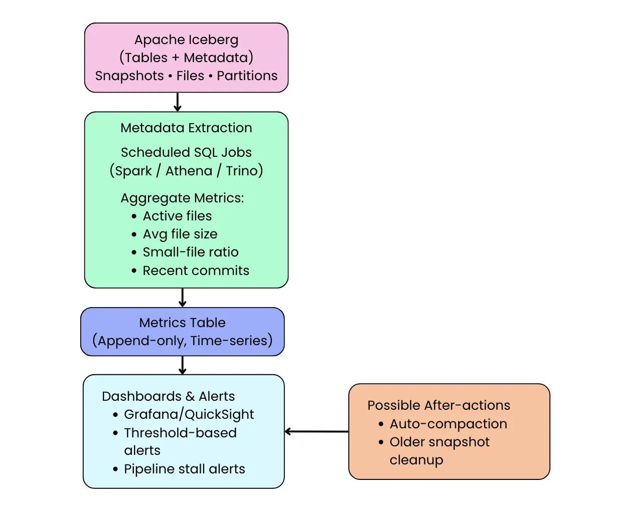
Operationalizing Observability: Pull (Metadata Queries) + Push (Metrics Reports)​

In production, Iceberg observability usually lands in two complementary patterns: pull-based monitoring via scheduled metadata queries, and push-based monitoring via runtime metrics reports. Pull-based monitoring is ideal when you want durable history for dashboards, trend analysis, capacity planning, and governance checks. Push-based monitoring is ideal when you need low-latency signals that react immediately to problematic writes or scans. Most teams end up using both, because together they provide a tight loop: detect anomalies, explain root cause using metadata tables, and trigger corrective action through alerts or maintenance jobs.

Pull-based monitoring: scheduled metadata queries​

The simplest and most common approach is to periodically query Iceberg’s metadata tables and materialize the results into a metrics store. Because metadata tables are transactional and safe to query continuously, teams often run a scheduled Spark job (every few minutes or hourly) that aggregates signals from tables like snapshots, files, and partitions. Those results are then appended into a separate metrics table or exported into a time-series backend.

SELECT
  date_trunc('hour', committed_at) AS window_start,
  COUNT(*) AS commits,
  SUM(CAST(summary['added-records'] AS BIGINT)) AS records_added,
  SUM(CAST(summary['added-files-size'] AS BIGINT)) AS bytes_added
FROM prod.db.orders.snapshots
WHERE committed_at >= current_timestamp() - INTERVAL 1 DAY
GROUP BY date_trunc('hour', committed_at)
ORDER BY window_start;

Push-based monitoring with Iceberg Metrics Reporters​

For near-real-time observability, Iceberg also supports a pluggable metrics reporting framework that emits runtime events such as CommitReport after table commits and ScanReport during query planning. These reports contain useful execution-time signals like the number and size of files added or removed, commit duration, retries, and scan planning characteristics. When wired into a monitoring system, these runtime events become an immediate detection layer that can catch bad commits as they happen rather than waiting for the next scheduled query. In practice, teams may start with logging-based reporting for validation, but production deployments typically forward the emitted events into Prometheus/OpenTelemetry/Datadog/CloudWatch pipelines using a dedicated reporter implementation. This push approach is especially valuable for event-driven automation, such as triggering compaction when average file sizes drop across consecutive commits or when delete files accumulate past a threshold.

How teams use both in practice​

In real systems, pull and push approaches complement each other rather than competing. A pragmatic setup is to treat push-based reports as the early warning system during active ingestion and heavy query periods, while pull-based queries provide the steady baseline for dashboards, audits, and longer-range planning. Together, they turn Iceberg’s metadata layer into a complete observability surface: you detect issues quickly, diagnose them precisely using metadata tables, and respond with targeted remediation rather than manual guesswork.

When push-based reporting is unavailable (for example, in certain catalog implementations), scheduled metadata queries remain the recommended approach. As Iceberg adoption grows, more catalogs and managed services are expected to support Metrics Reporters natively.

Ensuring a Performant and Reliable Data Lake​

By combining metadata queries with real-time metrics, Apache Iceberg empowers data engineers to build a robust observability and maintenance regime for data lakes. No longer do you have to treat the data lake as an opaque storage system with Iceberg, the table itself tells you about its health. You can catch problems like too many small files, unbalanced partitions, or unexpected schema changes early and address them proactively. The end result is a data lake that remains performant and reliable even as it scales, because potential issues are monitored and handled before they spiral out of control.

To put it succinctly in Iceberg’s own terms: metadata tables act like the observability layer for your data platform... You can use them to monitor pipeline health, detect anomalies before things break, audit changes over time, flag cost spikes, track freshness, and even automate alerts all with no extra tools, since it’s built into Iceberg. This is a paradigm shift from reactive to proactive data operations.

Comparison with Other Data Lake Table Formats​

It’s worth comparing Iceberg’s observability features to what’s available in other popular data lake table formats or traditional lakes:

• Apache Hive / Plain Data Lake: In traditional Hadoop/Hive-style lakes (or “plain” object storage layouts without a table format), operational visibility is often pieced together from a mix of metastore metadata and external inspection. The Hive Metastore can tell you about databases, tables, and partition locations, but it typically doesn’t provide a transactional history of changes or a complete, queryable view of file-level state (file counts, sizes, churn) without additional jobs or tooling. As a result, teams commonly rely on ad-hoc scripts to list files in HDFS/S3, engine-specific commands like SHOW PARTITIONS, and pipeline logs to infer what changed and when. Iceberg addresses this by storing richer table metadata as part of the table itself capturing snapshot history and exposing table state through queryable metadata structures so engineers can answer many of the same “what happened?” and “what does the table look like now?” questions more directly and consistently across engines that support Iceberg.
• Delta Lake: Delta Lake also improves observability compared to a plain data lake by maintaining a transaction log and exposing commit history through features like DESCRIBE HISTORY (or equivalent APIs), including details such as operation type and high-level commit metrics (e.g., files added/removed). In many setups, deeper file-level inspection like enumerating the exact set of active files or extracting detailed per-file stats is typically done by reading the transaction log and/or using Delta-specific APIs and tooling, and the exact experience can vary by platform. By contrast, Iceberg’s approach emphasizes exposing the table’s current physical state as queryable metadata tables (like table.files / table.partitions) in engines that support them, which can make it easier to do file-layout and partition-health analysis directly in SQL without additional log parsing.
• Apache Hudi: Apache Hudi has strong operational metadata and a mature commit timeline, and it supports pluggable metrics reporting (e.g., emitting commit and write metrics to common monitoring backends). In practice, engineers often inspect Hudi’s table state, commits, and file organization through Hudi’s own APIs, timeline/CLI tools, and platform-specific integrations, and the “SQL surface” for deep metadata can be more engine- and deployment-dependent. Iceberg’s advantage is that, where supported, many of the same operational questions (file counts, partition skew, delete-file buildup, recent table activity) can be answered via standardized, queryable metadata tables making ad-hoc inspection and dashboard extraction feel more uniform across compute engines.

In summary, Iceberg stands out by making metadata a first-class citizen of the data lake. As one blog noted, “unlike Hive or traditional file-based formats, where visibility depends on limited tooling, Iceberg exposes information as structured, queryable tables”. This design philosophy gives data engineers a uniform way to inspect and manage table health. While Delta and Hudi have their own strengths and do provide some monitoring capabilities, Iceberg’s comprehensive metadata tables and new metrics reporter framework offer an arguably more unified and flexible observability toolkit.

Conclusion​

Apache Iceberg brings much-needed observability to data lakes in a seamless, SQL-driven way. By introspecting table metadata, data engineers can monitor everything from file counts and sizes to schema changes and historical growth all using the same engines and tools they use for data queries. We saw how Iceberg’s metadata tables (history, snapshots, files, partitions, etc.) act as a built-in monitoring dashboard, and how new metrics reporters enable real-time alerts and automated maintenance. This means fewer surprises in production: you can catch issues like too many small files or an unexpected schema tweak before they wreak havoc on your pipelines. Iceberg essentially turns metadata into an “always-on” guardian of your data lake’s health.

For teams adopting Iceberg, the practical next step is to integrate these capabilities into your data operations. Build dashboards that track key Iceberg metrics, set up SQL-based alarms for anomalies, and consider enabling metrics reporters to tie into your observability stack. The goal is to ensure your data lake stays performant, reliable, and efficient as it scales and Iceberg provides the hooks to do exactly that. With a robust observability foundation, you can spend less time guessing what went wrong and more time optimizing and delivering value from your data.

In the end, Apache Iceberg exemplifies the evolution of data lakes towards being more self-describing and self-managing. Observability is not an afterthought but a core feature of the table format. For data engineers, this means easier troubleshooting, proactive maintenance, and confidence in the integrity and performance of their data platform. As the data ecosystem continues to grow, leveraging Iceberg’s monitoring and metrics features can be a game-changer in operating a modern, transparent data lake that you can trust.