Building a Data Lakehouse with Apache Iceberg + ClickHouse + OLake

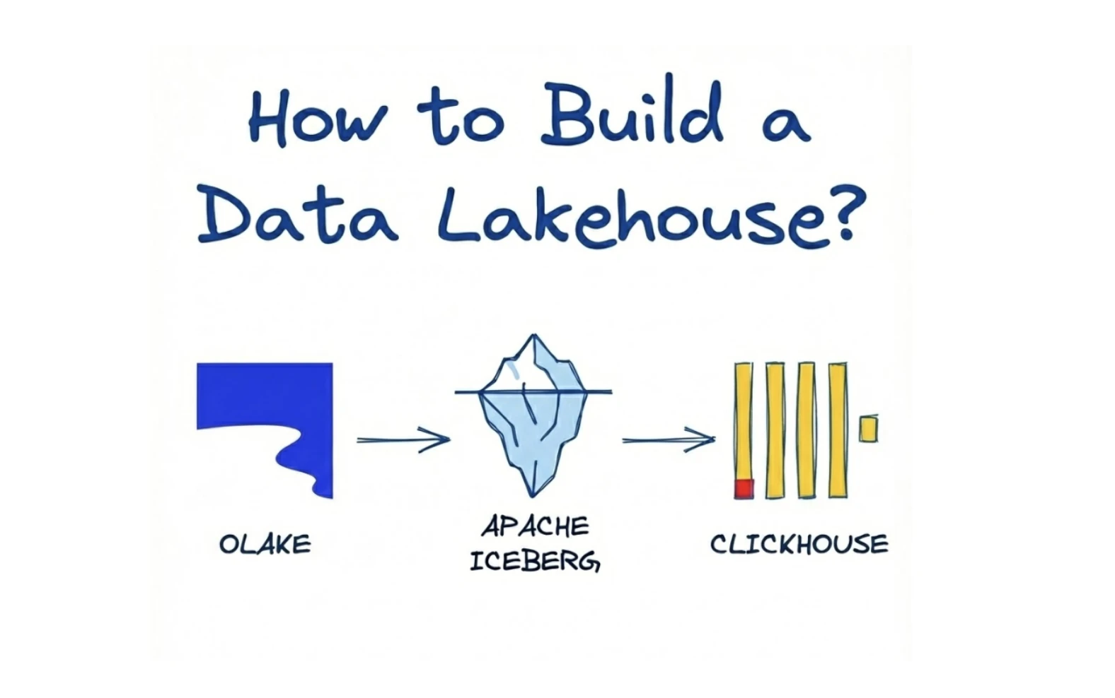
If you're serious about building a modern data architecture, you'll love this one. We'll put together a fully open-source lakehouse platform using Apache Iceberg, ClickHouse, OLake and MinIO — and you can spin it up on your laptop using Docker in a few steps.
What is a data lakehouse?
In short: it blends the flexibility of a data lake (large-scale object storage, schema-on-read) with the structure and performance of a data warehouse (transactions, fast queries, governance). With Iceberg as the table format, you get ACID semantics, schema evolution and time-travel out of the box. That means you can treat your object storage like a first-class table store, not just a dump of files.
Why this architecture matters
Here's the architecture we'll build:
-
Source: MySQL – the operational database
-
Ingestion: OLake UI captures CDC (change-data-capture) from MySQL and writes into Iceberg tables stored in MinIO
-
Storage: MinIO serves as the S3-compatible object storage for both raw and curated Iceberg tables
-
Metadata: Iceberg REST catalog (e.g., via PostgreSQL) tracks snapshots, schemas and manifests
-
Query engine: ClickHouse connects to the Iceberg REST catalog (via its DataLakeCatalog/Iceberg engine), enabling real-time analytics on data sitting in object storage
This architecture lets you move data from MySQL → Iceberg (raw) → queryable immediately in ClickHouse — without heavy ETL stacks, Kafka or massive orchestration overhead.
What we'll do
-
Set up OLake UI (as your orchestration hub for CDC pipelines)
-
Launch the core services: MySQL, MinIO, Iceberg REST catalog, ClickHouse — all via a single
docker compose up -dcommand -
In OLake UI: define a MySQL source (with CDC enabled), select MinIO/Iceberg as the destination, and activate a job (for example named
iceberg_job) which will write into a namespace likeiceberg_job_demo_dbon MinIO -
Map the Iceberg tables into ClickHouse using the Iceberg REST catalog and run analytics comparing raw Iceberg data with optimized Silver/Gold layers.
Table of Contents
- Architecture at a Glance
- Setting Up OLake UI - CDC Engine
- Clone the Repo & Understand the Layout
- Bring Up the Core Services
- MinIO Console - Your Data Lake Dashboard
- Seed MySQL with Demo Data
- 📊 Sample Data Overview
- Inspect MySQL Data Before Syncing
- Prepare ClickHouse for the Iceberg REST Catalog
- Configure OLake UI: Step-by-Step Guide
- Query Iceberg Tables from ClickHouse
- Understanding the Three-Layer Architecture
- Raw vs Optimized Analytics & Performance Comparison
- Cleaning Up the Environment
- Where to Go Next
Architecture at a Glance
The following diagram illustrates the complete data flow from MySQL through OLake CDC, into MinIO as Iceberg tables, and finally into ClickHouse for analytics:
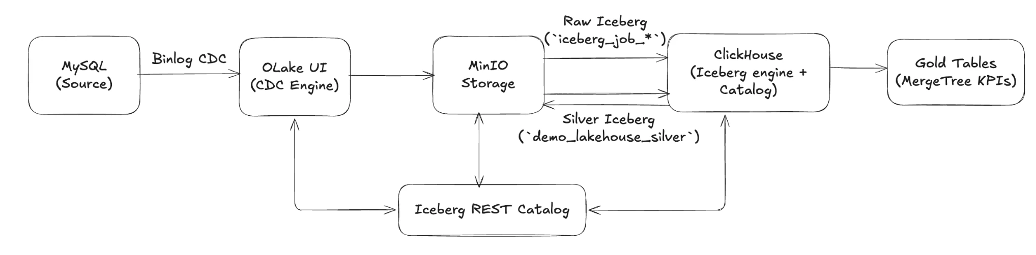
How the pieces work together
-
MySQL emits change events via binlog. OLake UI captures those CDC streams and lands them in MinIO as raw Iceberg tables under the namespace
iceberg_job_<database>. -
Iceberg REST Catalog keeps the table metadata (schemas, snapshots, manifests) in PostgreSQL while pointing all data files to MinIO's
warehousebucket. -
ClickHouse connects to the REST catalog using the
DataLakeCatalogengine, which lets it read the raw Iceberg tables, build an optimized Silver Iceberg table back in MinIO, and materialize Gold KPIs in local MergeTree storage.
Key components
-
MySQL 8.0 – Demo OLTP workload with GTID + binlog enabled for OLake CDC.
-
OLake UI (separate docker-compose) – Configures the source, destination, and
iceberg_jobpipeline that writes Iceberg tables to MinIO through the REST catalog. -
MinIO – Acts as the S3-compatible warehouse holding both the raw namespace (
iceberg_job_demo_db) and the curated Silver namespace (demo_lakehouse_silver). -
Iceberg REST Catalog + PostgreSQL – Serves metadata to both OLake and ClickHouse, ensuring all engines see the same table definitions.
-
ClickHouse – Queries raw Iceberg via REST, writes the Silver Iceberg table back to MinIO, and stores Gold aggregates locally for sub-10ms dashboards.
Setting Up OLake UI - CDC Engine
OLake has one of its unique offerings the OLake UI, which we will be using for our setup. This is a user-friendly control center for managing data pipelines without relying heavily on CLI commands. It allows you to configure sources, destinations, and jobs visually, making the setup more accessible and less error-prone. Many organizations actively use OLake UI to reduce manual CLI work, streamline CDC pipelines, and adopt a no-code-friendly approach.
For our setup, we will be working with the OLake UI. We'll start by cloning the repository from GitHub and bringing it up using Docker Compose. Once the UI is running, it will serve as our control hub for creating and monitoring all CDC pipelines.
Let's start by getting the interface running. Go ahead and create a folder named olake-setup. Inside this folder, create another folder called olake-data.
mkdir olake-setup
cd olake-setup
mkdir olake-data
Clone the OLake UI repository:
git clone https://github.com/datazip-inc/olake-ui.git
Now, here's the important part - open up the docker-compose file you would see a persistence path command there. We need to make sure the persistence path is set correctly. Otherwise, you'll lose all your configurations every time you restart the containers.
Make sure to run this command in your terminal so it saves your file location for the host persistence path (while still in the olake-setup directory, before changing into olake-ui):
export PWD=$(pwd)
cd olake-ui
The OLake UI docker-compose file uses ${PWD}/olake-data as the host persistence path. This means all your OLake configurations, job states, and metadata will be saved to an olake-data folder in your current directory. Well, that's exactly what we want - persistent storage that survives container restarts!
Now let's fire up the OLake UI:
docker compose up -d
Once it's running, go ahead at http://localhost:8000, olake-ui and use these credentials:
-
Username:
admin -
Password:
password
You are greeted with Olake UI! The dashboard will show you job status tabs and an onboarding tutorial to help you get started.
Note: Keep this terminal window open or note the directory path. You'll need to come back to this OLake UI setup later when configuring your pipelines. For now, let's set up the rest of the infrastructure.
Clone the Repo & Understand the Layout
Now, let's set up the main lakehouse infrastructure. In a new terminal window (or navigate to a different directory), clone the main repository:
git clone https://github.com/sandeep-devarapalli/Apache-Iceberg-with-clickhouse-olake.git
cd Apache-Iceberg-with-clickhouse-olake
tree -F -L 1
Directory highlights:
-
docker-compose.yml– orchestrates core services (MySQL, MinIO, ClickHouse, Iceberg REST Catalog, helper clients). Note: This does NOT include OLake UI - we set that up separately above. -
mysql-init/– DDL + seed data executed automatically for the demo schema. -
clickhouse-config/– server + user configs that enable the Iceberg feature flags. -
scripts/– SQL helpers (mysql-integration.sqlnow acts as an Iceberg REST smoke test, plusiceberg-setup.sql&cross-database-analytics.sql).
Bring Up the Core Services
Start the core services (MySQL, MinIO, ClickHouse, and Iceberg REST Catalog). Note: OLake UI is already running separately from the previous step.
docker compose up -d
docker compose ps
What to expect:
-
All services will start and become healthy within 1-2 minutes
-
The
mccontainer will create thewarehouseandolake-databuckets and then exit with status 0 (this is normal - the container's job is done) -
The
init-test-tablecontainer will create a test table (test_olake.test_olake) for OLake connection testing and then exit (this ensures OLake's test connection succeeds) -
You should see all core services (mysql, minio, postgres, iceberg-rest, clickhouse) showing "healthy" status
-
The
olake-auto-connectservice will start and keep running to connect OLake test containers to the network
Verification after startup:
# Verify REST Catalog is accessible
curl http://localhost:8181/v1/config
# Should return: {"defaults":{},"overrides":{}}

# Check that buckets were created (check mc logs)
docker ps -a --filter "name=mc" --format "{{.ID}}" | head -1 | xargs -I {} docker logs {} 2>&1 | grep -E "(warehouse|complete)"

# Verify test table was created for OLake connection testing
docker logs init-test-table
# Should show: "✅ Test table created successfully! OLake test connection should now work."

# Verify test table exists in REST catalog
curl -s http://localhost:8181/v1/namespaces/test_olake/tables | jq .
# Should show: {"identifiers":[{"namespace":["test_olake"],"name":"test_olake"}]}
| Service | Purpose | Host Access |
|---|---|---|
mysql-server | Source OLTP DB | localhost:3307 |
postgres | Iceberg REST catalog metadata storage | localhost:5432 |
minio | S3-compatible storage | API http://localhost:9090, Console http://localhost:9091 |
mc | MinIO client for bucket initialization | Creates warehouse and olake-data buckets, then exits (this is expected) |
clickhouse-server | Query engine | HTTP http://localhost:8123, Native localhost:19000 |
clickhouse-client, mysql-client | Utility containers | used for scripts |
iceberg-rest | Iceberg REST catalog | REST API http://localhost:8181 |
olake-auto-connect | Network connector | Automatically connects OLake test containers to the Docker network |
Note: OLake UI and its dependencies (PostgreSQL, Temporal, Elasticsearch) are running separately in the olake-setup/olake-ui directory we set up earlier. Access it at http://localhost:8000.
MinIO Console - Your Data Lake Dashboard
Once MinIO is running, you can access the MinIO Console to visually inspect your data lake:
Access the MinIO Console:
-
URL:
http://localhost:9091 -
Username:
admin -
Password:
password
The MinIO Console provides a web-based interface where you can:
-
Browse buckets and objects
-
Monitor storage usage
-
Verify that Iceberg tables are being written correctly
-
Inspect the
warehousebucket structure
The warehouse and olake-data buckets are automatically created by the mc service in docker-compose.yml.
Note: The mc container exits after successfully creating the buckets (exit code 0) - this is expected behavior. You can verify the buckets exist by checking the MinIO Console (http://localhost:9091) or by checking the mc container logs. Once OLake starts writing data, you'll see directories for each table (e.g., iceberg_job_demo_db/users/, iceberg_job_demo_db/products/, etc.) containing Iceberg metadata and Parquet data files. The namespace format is <job_name>_<database_name>.
Seed MySQL with Demo Data
The MySQL container automatically executes:
-
mysql-init/01-setup.sql– creates thedemo_dbschema (users,products,orders,user_sessions) and automatically generates a large dataset for performance testing:-
~1000 users with realistic demographics across 13 countries
-
~200 products across 9 categories
-
~10,000 orders (approximately 10 orders per user)
-
~5,000 user sessions (approximately 5 sessions per user)
-
-
mysql-init/02-permissions.sql– creates integration users:-
olake / olake_pass(CDC + replication privileges for OLake UI). -
demo_user / demo_password(for manual testing and inspection).
-
📊 Sample Data Overview
The demo includes realistic e-commerce data:
Tables:
-
users (1000+ users) - Customer information with demographics
-
products (200+ products) - Product catalog across multiple categories
-
orders (10,000+ orders) - Purchase history with various statuses
-
user_sessions (5,000+ sessions) - User activity tracking
Geographic Distribution:
USA, Canada, UK, Germany, France, Spain, Japan, India, Australia, Norway, Brazil, Mexico, Singapore
Product Categories:
Electronics, Gaming, Software, Home, Health, Books, Education, Accessories, Furniture
Inspect MySQL Data Before Syncing
Before configuring OLake UI, you may want to inspect what data is available in MySQL.
Quick script (recommended):
# Run the helper script for a complete overview
./scripts/inspect-mysql-data.sh
Prepare ClickHouse for the Iceberg REST Catalog
ClickHouse ships with experimental Iceberg support disabled by default. The repo already enables the necessary flags inside clickhouse-config/config.xml and expects an Iceberg REST catalog provided by OLake.
Iceberg REST Catalog Details:
-
REST Catalog URI (for OLake UI):
http://host.docker.internal:8181(use this in OLake destination configuration) -
REST Catalog URI (from host):
http://localhost:8181(for testing from your machine) -
Full API endpoint:
http://localhost:8181/v1/config(for health checks from host) -
Namespace:
iceberg_job_demo_db(format:<job_name>_<database_name>- where OLake writes the raw Iceberg tables) -
No authentication required (Iceberg REST catalog doesn't use auth by default)
The Iceberg REST catalog service (iceberg-rest) is included in docker-compose.yml and provides the REST API for Iceberg table metadata. It uses a PostgreSQL-backed catalog (the postgres service) for persistent metadata storage, ensuring catalog state survives container restarts. The actual Iceberg table data is stored in MinIO's warehouse bucket and persists independently.
Once the container is healthy (check with docker-compose ps), you can proceed with the OLake pipeline steps.
Configure OLake UI: Step-by-Step Guide
OLake UI should already be running from the earlier setup step.
Now let's configure OLake UI to replicate data from MySQL to Iceberg tables in MinIO. Open your browser and navigate to http://localhost:8000. You'll see the OLake UI login page.
Note: OLake UI runs in a separate Docker Compose setup and connects to the core services (MySQL, MinIO, etc.) via host.docker.internal or container IP addresses. The core services should be running from the previous step.
Step 1: Log in to OLake UI
-
URL:
http://localhost:8000 -
Username:
admin -
Password:
password
Once logged in, you'll see the OLake dashboard. We need to configure two things: a Source (MySQL) and a Destination (Iceberg on MinIO).
Step 2: Register the MySQL Source
-
In the left sidebar, click on Sources, then click New Source.
-
Select MySQL as the source type.
-
Fill in the connection details:
-
Name of your source:
mysql_source(or a descriptive name of your choosing) -
OLake Version: latest
-
Host:
host.docker.internal(use this to access MySQL via host port mapping, or usemysqlif OLake UI is on the same Docker network) -
Port:
3307(use the host port if usinghost.docker.internal, or3306if using Docker service namemysql) -
Database:
demo_db -
Username:
olake -
Password:
olake_pass -
Enable SSL: Leave this unchecked (set to
false) -
Sync Mode:
Full Refresh(default) -
Ingestion Mode:
Upsert(default)
-
-
Click Next or Test Connection to verify the connection works.

Great! Your MySQL source is now registered.
Step 3: Register the Iceberg Destination (MinIO) using OLake REST Catalog
-
In the left sidebar, click on Destinations, then click New Destination.
-
Select Apache Iceberg as the destination type.
- Name of your destination:
iceberg_destination(or a descriptive name of your choosing)
- Name of your destination:
-
In the Catalog section:
-
Catalog: Select
REST Catalog -
REST Catalog URI:
http://host.docker.internal:8181(use host.docker.internal to access services via host port mappings) -
S3 Path:
s3://warehouse/(this is the S3 path where Iceberg tables will be stored) -
S3 Endpoint:
http://host.docker.internal:9090(use host.docker.internal with host port 9090, which maps to MinIO's container port 9090) -
AWS Access Key:
admin(MinIO access key) -
AWS Secret Key:
password(MinIO secret key) -
AWS Region:
us-east-1
-
-
Click Save or Create Destination.
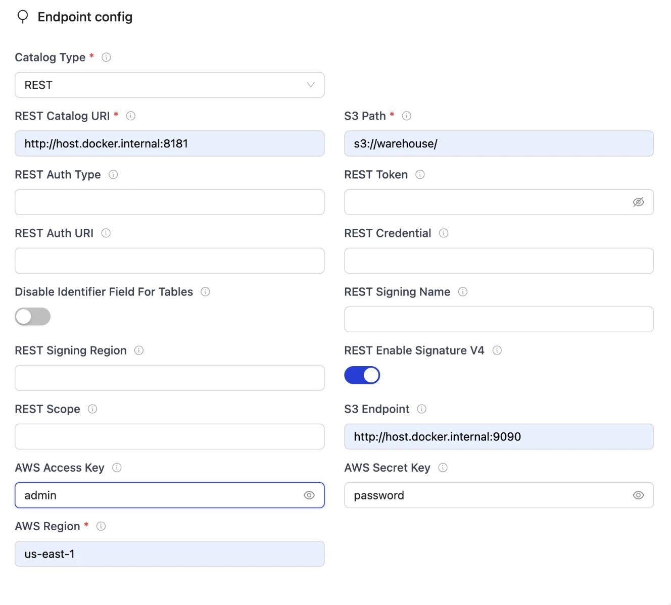
Perfect! Now OLake knows where to write the Iceberg tables.
The destination is configured to use:
-
Iceberg REST Catalog at
http://host.docker.internal:8181for catalog metadata (accessed via host port mapping) -
MinIO at
http://host.docker.internal:9090as the S3-compatible storage backend (accessed via host port mapping - host port 9090 maps to MinIO's container port 9090) -
S3 Bucket:
warehouse(automatically created by themcservice) -
Namespace: The namespace will be automatically created based on your job name and database (format:
<job_name>_<database_name>). For example, if your job is namediceberg_joband your MySQL database isdemo_db, the namespace will beiceberg_job_demo_db.
Step 4: Create and Configure the Pipeline
Now we'll create a pipeline that connects the MySQL source to the Iceberg destination. You can create a single multi-table pipeline (recommended for this demo)
-
In the left sidebar, click on Jobs, then click New Job or Create Job.
-
Name your job:
iceberg_job(or any name you prefer - this will be used as part of the namespace) -
Select your MySQL source (the one you just created).
-
Select your Iceberg destination (the one you just created).
-
Configure per-table settings. For each table, set the partition strategy using Iceberg partition transforms:
Table Partition Regex Primary Key Use Case users/{created_at, month}/{country, identity}idMonthly user analytics with geographic filtering products/{category, identity}idCategory-based product queries orders/{order_date, month}/{status, identity}idMonthly order reporting by status user_sessions/{login_time, day}idDaily session analytics Understanding Iceberg Partition Transforms:
Iceberg partitioning groups rows that share common values at write-time, enabling efficient query pruning. When you filter on partition columns, Iceberg consults metadata to skip irrelevant data files entirely.
Transforms used in this demo:
-
month(created_at): Extracts the month (1-12) from a timestamp. Ideal for monthly reporting and time-range queries. -
day(login_time): Returns the calendar day (1-31) from a timestamp. Perfect for daily dashboards and retention policies. -
identity(country): Writes the raw column value unchanged. Best for columns with few distinct values like country, status, or category.
Why these partitions?
-
userstable: Partitioned by month and country enables efficient queries like "users created in January from USA" - Iceberg scans only thecreated_at_month=1/country=USA/directory. -
productstable: Identity transform on category allows category-based analytics to skip irrelevant product types. -
orderstable: Month + status partitioning optimizes queries like "orders in April with status 'shipped'" - scans onlyorder_date_month=4/status=shipped/data. -
user_sessionstable: Daily partitioning enables efficient time-range queries for session analytics and daily dashboards.
How to configure in OLake UI:
-
Select your table in the job configuration
-
Keep Normalization enabled
-
Select Partitioning in the right tab
-
Enter the partition regex in the format:
/{field_name, transform} -
For hierarchical partitioning (multiple levels), use:
/{field1, transform1}/{field2, transform2} -
Set Sync Mode:
Full Refresh(default) -
Set Ingestion Mode:
Upsert(default)
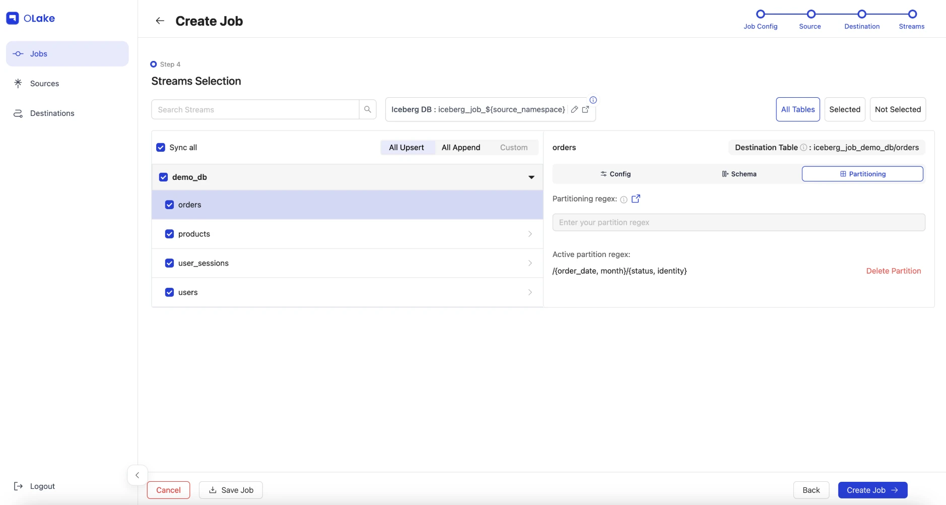
Example: For the
userstable, enter:/{created_at, month}/{country, identity}Important Notes:
-
Iceberg does not support redundant fields during partitioning. Avoid applying multiple time transforms to the same column (e.g., don't use both
year(ts)andmonth(ts)on the same column). -
Start simple and evolve: You can add more partition fields later as your query patterns change. Iceberg maintains backward compatibility with old snapshots.
-
Aim for 100-10,000 files per partition folder for optimal performance.
-
-
Click Save.
Step 5: Start the Job and Watch It Run
-
Find your job (named
iceberg_job) in the Jobs list and click on it. -
Click Sync now under the Actions button.
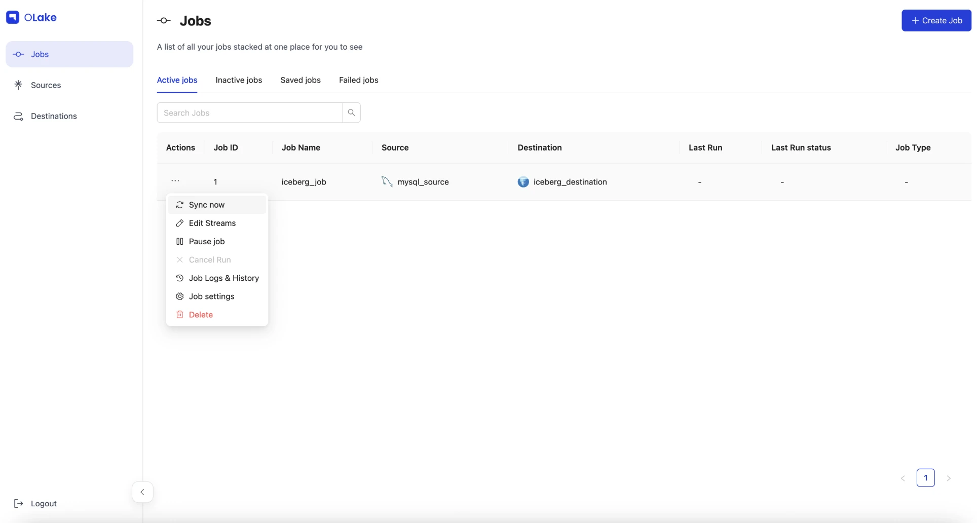
That's it! OLake will now start syncing your MySQL data to Iceberg tables. Here's what happens behind the scenes:
-
OLake takes an initial snapshot of all data from MySQL (this may take 2-5 minutes with 10,000+ orders)
-
It creates Iceberg tables in the namespace
iceberg_job_demo_db(format:<job_name>_<database_name>) -
Data gets written to MinIO as Parquet files organized by your partition strategy
-
Once the initial sync completes, the job continues running to capture any new changes via CDC
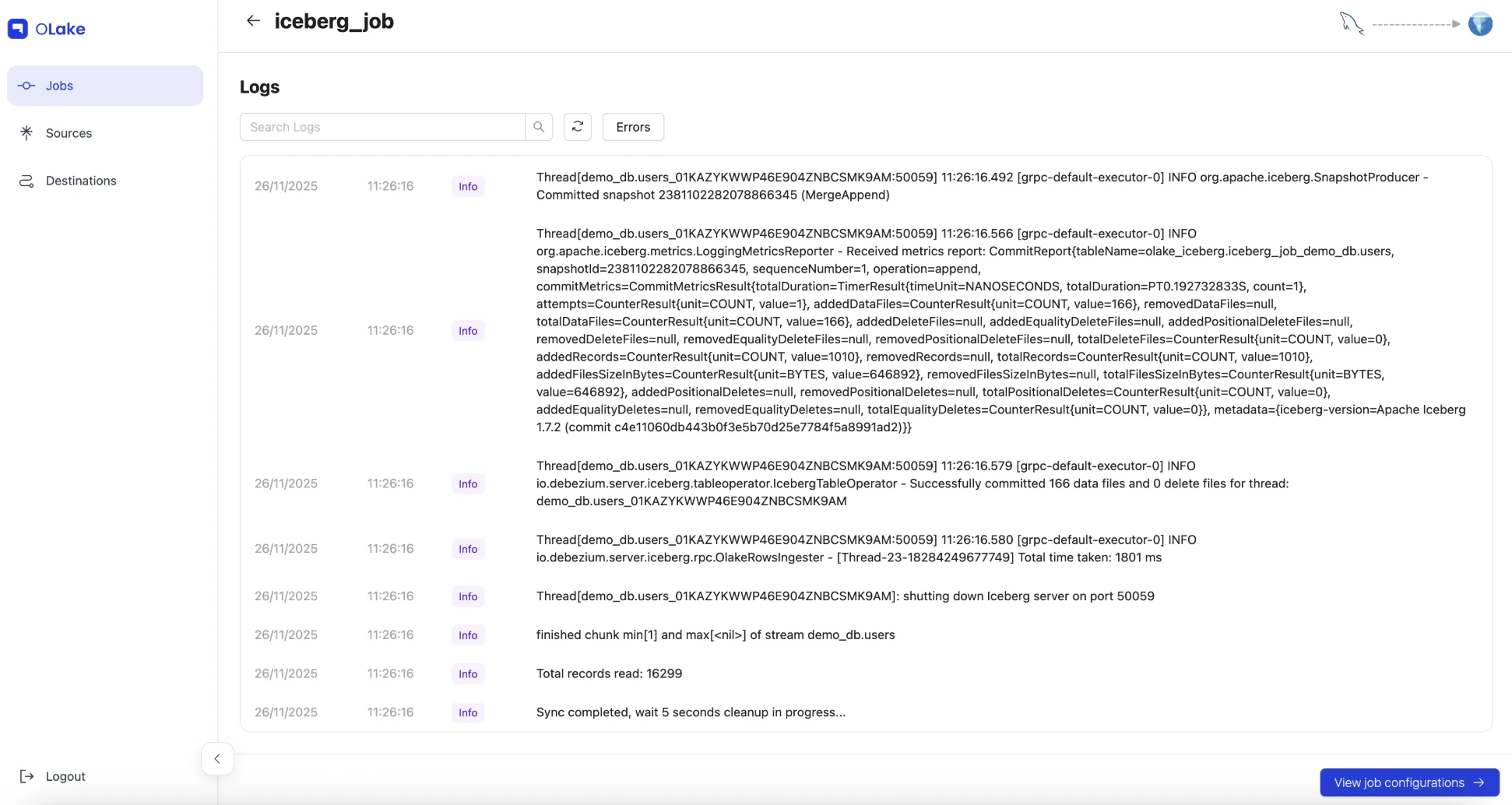
Watch the logs in real-time:
While the job is running, you can watch the progress in OLake UI. The logs will show messages like:
-
"Creating destination table [table_name] in Iceberg database [iceberg_job_demo_db]"
-
"Successfully wrote X events for thread"
-
"Successfully committed X data files"
-
"Sync completed"
When you see "Sync completed" in the logs, the initial snapshot is done! The job will keep running to capture any future changes from MySQL.
Verify Everything Worked
Once the sync completes, let's make sure all your data made it through correctly. You can verify in two ways:
1. Check the row counts in OLake UI:
Click on your job (iceberg_job) and check the monitoring/status tab. You should see approximately:
-
~1,010 users (committed as 167 data files)
-
~115 products (committed as 9 data files)
-
~10,115 orders (committed as 65 data files)
-
~5,059 user sessions (committed as 30 data files)
-
Total: ~16,299 records synced successfully
2. Verify the Iceberg tables exist in MinIO:
The easiest way is through the MinIO Console:
-
Open
http://localhost:9091in your browser -
Login with
admin/password -
Navigate to the
warehousebucket →iceberg_job_demo_db/namespace -
You should see four table directories:
users/,products/,orders/,user_sessions/

Each table directory contains:
-
metadata/folder with Iceberg metadata files (snapshots, manifests, schema) -
data/folder with Parquet files organized by partition
For example, the orders/ table will have partition folders like:
-
data/order_date_month=2024-11/status=pending/ -
data/order_date_month=2024-11/status=shipped/ -
data/order_date_month=2024-12/status=confirmed/
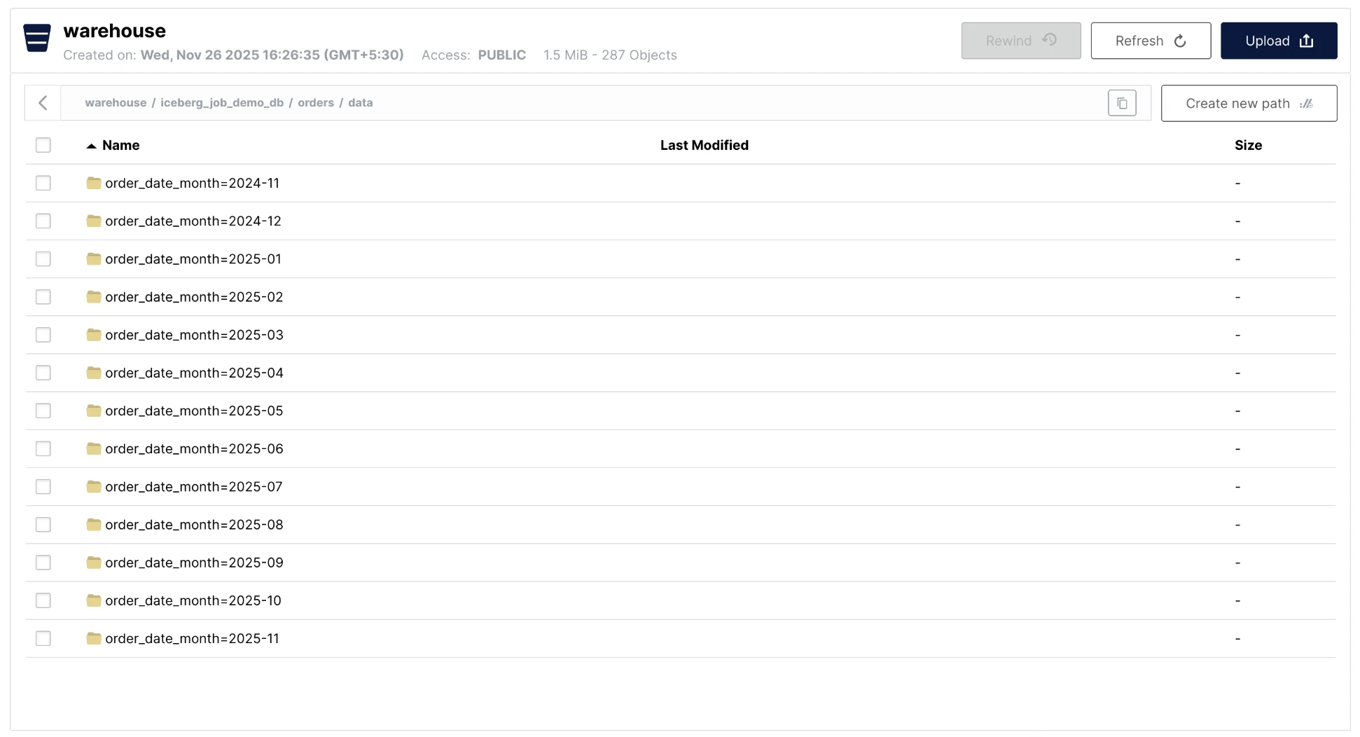
This partition structure is what makes queries fast - when ClickHouse filters on partition columns, it only reads the relevant folders instead of scanning everything.
Alternative: Check via command line:
If you prefer the command line, you can use the MinIO client:
# List all tables in your namespace
docker run --rm --network apache-iceberg-with-clickhouse-olake_clickhouse_lakehouse-net \
  -e MC_HOST_minio=http://admin:password@minio:9090 \
  minio/mc ls minio/warehouse/iceberg_job_demo_db/

# Should show: orders/, products/, user_sessions/, users/
Once you've verified the data is there, you're ready to query it with ClickHouse!
Query Iceberg Tables from ClickHouse
Now that OLake has written the Iceberg tables to MinIO, let's connect ClickHouse to query them. ClickHouse uses the DataLakeCatalog engine to connect to the Iceberg REST catalog.
How it works:
ClickHouse connects to the REST catalog by creating a database (not individual tables) using the DataLakeCatalog engine. This database provides access to all tables in the specified namespace, and you query them through the database connection.
Step-by-Step Setup:
We've broken down the setup into three separate scripts so you can verify each step:
Step 1: Query Raw Iceberg Tables
First, verify that ClickHouse can connect to and query the raw Iceberg tables written by OLake:
docker exec -it clickhouse-client clickhouse-client --host clickhouse --time --queries-file /scripts/iceberg-query-raw.sql
This script will:
-
Create a database connection to the REST catalog using
DataLakeCatalogengine -
List all available tables in the catalog
-
Query the raw Iceberg tables (users, products, orders, user_sessions) and show row counts
-
Display sample data to verify the connection works
Important: The script uses iceberg_job_demo_db as the default namespace (matching the job name iceberg_job from our example). If you used a different job name, you'll need to update the warehouse setting in the script (scripts/iceberg-query-raw.sql) to match your actual namespace. The namespace format is <job_name>_<database_name>.
Understanding the timing and caching:
When you run this script, you'll notice something interesting about the timing:
-
First query (
SHOW TABLES): Takes 30-70 seconds-
This is the initial setup where ClickHouse connects to the REST catalog
-
It fetches metadata for all tables (schema, partitions, file locations)
-
This metadata is cached in memory for the database connection
-
-
Subsequent queries in the same run: Very fast (0.001-0.018 seconds)
-
Once metadata is cached, queries are nearly instant
-
ClickHouse uses the cached metadata to locate and read Parquet files
-
-
Why re-running the script takes 30-70 seconds again:
-
The script includes
DROP DATABASE IF EXISTSwhich destroys the database connection -
This clears the metadata cache, so the next run must fetch everything again
-
This is intentional - it ensures a clean state for testing
-
To see caching in action:
If you want to experience the speed of cached queries, keep the database connection alive:
# Step 1: Run the script once (this creates the database and caches metadata)
docker exec -it clickhouse-client clickhouse-client --host clickhouse --queries-file /scripts/iceberg-query-raw.sql

# Step 2: Now run individual queries without dropping the database
# These will be fast because the metadata is cached!
docker exec -it clickhouse-client clickhouse-client --host clickhouse --time --query "
USE demo_lakehouse_db;
SELECT COUNT(*) FROM \`iceberg_job_demo_db.users\`;
"

# You'll see this query completes in milliseconds (0.001-0.006 seconds)
# because the database connection and metadata cache are still alive!
You will see the response like:
0.001    <- Execution time for "USE demo_lakehouse_db;" (1 millisecond)
1010     <- Result of "SELECT COUNT(*) FROM `iceberg_job_demo_db.users`;"
0.008    <- Execution time for the SELECT query (8 milliseconds)
What the delay means:
The 30-70 second delay for SHOW TABLES is normal and happens because:
-
ClickHouse establishes a connection to the REST catalog API (
http://iceberg-rest:8181/v1) -
It makes API calls to fetch metadata for each table in the namespace
-
This metadata includes table schemas, partition information, and S3 file locations
-
All this metadata is then cached in memory for fast subsequent queries
This is a one-time cost per database connection. In production, you'd typically keep the database connection alive, so you'd only pay this cost once when the connection is first established.
Expected output from Step 1:
When you run Step 1, you should see output similar to this.
0.001
0.000
0.000
0.001
0.002
0.001
=== Available tables in REST catalog ===
0.001
iceberg_job_demo_db.orders
iceberg_job_demo_db.products
iceberg_job_demo_db.user_sessions
iceberg_job_demo_db.users
test_olake.test_olake
65.507
=== Raw Iceberg Table Row Counts ===
0.001
Iceberg users rows	1010
0.006
Iceberg products rows	115
0.005
Iceberg orders rows	10115
0.004
Iceberg user_sessions rows	5059
0.004
=== Sample Data Verification ===
0.000
Sample users (first 5):
0.000
78	user_47	user_47@example.com	Canada
374	user_343	user_343@example.com	Canada
584	user_533	user_533@example.com	Canada
703	user_612	user_612@example.com	Canada
795	user_724	user_724@example.com	Canada
0.007
Sample orders by status:
0.000
pending	2033
shipped	2002
delivered	2009
cancelled	2031
confirmed	2040
0.018
=== Step 1 Complete: Raw tables are accessible ===
0.001
You can now proceed to Step 2: Create Silver Layer
0.001
Step 2: Create Silver Layer (Optimized Iceberg table in MinIO)
Before ClickHouse can write data to the silver table, you need to create the empty Iceberg table structure in the REST catalog. This is a one-time prerequisite:
./scripts/create-silver-iceberg-table.sh
This script:
-
Ensures the
demo_lakehouse_silvernamespace exists -
Creates the empty
orders_curatedIceberg table with the schema/partitioning that will be used by the silver layer
Now populate the silver table with curated data:
docker exec -it clickhouse-client clickhouse-client --host clickhouse --queries-file /scripts/iceberg-create-silver.sql
This script will:
-
Attach ClickHouse to the empty Iceberg table you just created (via the named collection)
-
Enable experimental Iceberg inserts
-
Read from the raw Iceberg tables (
demo_lakehouse_db) -
Populate the silver Iceberg table in MinIO (
demo_lakehouse_silver.orders_curated) with curated data -
Show sample queries against the populated silver Iceberg table
Expected output:
When you run this script, you should see output similar to this:
=== Creating Silver Layer in MinIO (Iceberg) ===
=== Inserting optimized data into silver Iceberg table ===
This reads raw Iceberg (MinIO) and writes a curated Iceberg table (MinIO)...
=== Silver Layer Created Successfully (Iceberg in MinIO) ===
Silver orders rows (Iceberg)	10115
=== Querying Silver Table ===
pending	2033	3898.21
shipped	2002	4030.08
delivered	2009	4013.35
cancelled	2031	3968.85
confirmed	2040	4150.1
=== Location Note ===
Silver layer is an Iceberg table stored in MinIO (demo_lakehouse_silver/orders_curated).
=== Step 2 Complete: Silver layer created in MinIO ===
You can now proceed to Step 3: Create Gold Layer
Understanding the output:
-
"Silver orders rows (Iceberg) 10115": This confirms that all 10,115 orders from the raw layer were successfully written to the silver Iceberg table in MinIO. The data transformation (selecting specific columns, converting
order_datetoorder_month, etc.) completed successfully. -
The query results table shows order statistics grouped by status:
-
First column: Order status (pending, shipped, delivered, cancelled, confirmed)
-
Second column: Count of orders per status (approximately 2,000 orders per status, totaling ~10,115)
-
Third column: Average order value per status (ranging from ~$3,900 to ~$4,150)
-
-
"Silver layer is an Iceberg table stored in MinIO": This confirms the silver table is stored as an Iceberg table in MinIO, making it accessible to any Iceberg-compatible engine (Spark, Dremio, Trino, etc.), not just ClickHouse.
Why this is powerful:
-
End-to-end Iceberg: Both raw and silver layers live in MinIO as Iceberg tables
-
ClickHouse as an Iceberg writer: You can reuse the Iceberg tables across engines (Spark, Dremio, Trino, etc.)
-
Optimal layout: The silver table stores curated columns with identity partitions on
order_monthandstatus -
Data transformation: The silver layer contains only the columns needed for analytics, with optimized data types and partitioning for faster queries
Step 3: Create Gold Layer (Pre-aggregated KPIs)
Finally, create the gold layer with pre-aggregated metrics stored locally in ClickHouse for fastest queries:
docker exec -it clickhouse-client clickhouse-client --host clickhouse --queries-file /scripts/iceberg-create-gold.sql
This script will:
-
Create a local MergeTree table for pre-aggregated KPIs
-
Aggregate data from the silver layer
-
Display sample metrics
Expected output:
When you run this script, you should see output similar to this:
=== Creating Gold Layer (Pre-aggregated KPIs) ===
=== Aggregating data from Silver layer (Iceberg in MinIO) ===
=== Gold Layer Created Successfully ===
Gold metrics rows	1818
=== Sample Gold Metrics ===
2025-11-23	cancelled	7	7	18799.46	2685.64
2025-11-23	confirmed	7	7	17735.85	2533.69
2025-11-23	delivered	13	15	33020.78	2201.39
2025-11-23	pending	7	7	33032.51	4718.93
2025-11-23	shipped	7	7	10386.81	1483.83
2025-11-22	cancelled	6	6	33598.61	5599.77
2025-11-22	confirmed	4	4	7718.21	1929.55
2025-11-22	delivered	4	4	10067.03	2516.76
2025-11-22	pending	4	4	16590.89	4147.72
2025-11-22	shipped	7	7	13980.62	1997.23
=== All Layers Summary ===
Raw Iceberg (MinIO): demo_lakehouse_db.`iceberg_job_demo_db.*`
Silver Iceberg (MinIO): default.silver_orders_iceberg
Gold Metrics (Local): default.ch_gold_order_metrics
=== Step 3 Complete: Gold layer created ===
All three layers are now ready for querying!
Understanding the output:
-
"Gold metrics rows 1818": This confirms that 1,818 pre-aggregated metric rows were created. Each row represents a unique combination of
order_monthandstatus, with pre-computed KPIs (user count, order count, gross revenue, average order value). This is much smaller than the 10,115 raw orders because it's aggregated. -
The sample gold metrics table shows pre-computed KPIs for different months and statuses:
-
First column:
order_month(Date) - The month of the orders -
Second column:
status- Order status (cancelled, confirmed, delivered, pending, shipped) -
Third column:
user_count- Number of unique customers for that month/status combination -
Fourth column:
order_count- Total number of orders for that month/status -
Fifth column:
gross_revenue- Total revenue (sum of all order amounts) -
Sixth column:
avg_order_value- Average order value (gross_revenue / order_count)
-
-
"All Layers Summary": This confirms all three layers are now accessible:
-
Raw: Original Iceberg tables in MinIO (written by OLake)
-
Silver: Optimized Iceberg table in MinIO (written by ClickHouse)
-
Gold: Pre-aggregated metrics in ClickHouse local storage (fastest queries)
-
-
Why this is powerful: The gold layer enables instant dashboard queries. Instead of aggregating 10,115 orders every time, you can query pre-computed metrics in milliseconds. For example, to get "total revenue by status in November 2025", ClickHouse just reads the pre-aggregated rows instead of scanning and summing thousands of orders.
Understanding the Three-Layer Architecture
The data architecture uses three layers for optimal performance:
-
Raw Iceberg tables (in MinIO) - Written by OLake from MySQL
-
Namespace:
iceberg_job_demo_db(format:<job_name>_<database_name>) -
Unoptimized layout, all columns, original partitioning
-
-
Silver Iceberg tables (in MinIO) - Written by ClickHouse back to MinIO
-
Table:
default.silver_orders_iceberg(ClickHouse table alias pointing to MinIO) -
Actual data stored in: MinIO (
demo_lakehouse_silver/orders_curated) -
How it works:
silver_orders_icebergis a ClickHouse table definition (in thedefaultdatabase) that uses theIcebergengine to reference the actual Iceberg table stored in MinIO. Think of it as a "view" or "alias" - the table definition lives in ClickHouse, but all the data is stored in MinIO as an Iceberg table. -
ClickHouse optimizes with curated columns, identity partitions, and Iceberg metadata
-
Faster than raw because it's curated and still accessible to any Iceberg-compatible engine
-
Loaded from raw Iceberg tables and optimized for common query patterns
-
-
Gold tables (in ClickHouse local storage) - Pre-aggregated KPIs
-
ch_gold_order_metrics– aMergeTreetable with pre-computed metrics -
Fastest queries, no computation needed
-
The setup scripts create:
-
Raw layer: Tables accessible via
demo_lakehouse_dbdatabase (e.g.,`iceberg_job_demo_db.users`) - stored in MinIO as Iceberg tables -
Silver layer:
default.silver_orders_iceberg– an optimized Iceberg table in MinIO (demo_lakehouse_silver.orders_curated) written by ClickHouse -
Gold layer:
default.ch_gold_order_metrics– a per-month, per-status aggregate in ClickHouse local storage
Why this architecture matters:
-
Raw Iceberg: Proves ClickHouse can read OLake-managed data, but queries are slower due to unoptimized layout and network I/O from MinIO
-
Silver: ClickHouse writes an optimized Iceberg table back to MinIO with curated columns and identity partitions. Queries are faster than raw because of the optimized schema and partitioning, but still require network I/O to MinIO. The table is accessible to any Iceberg-compatible engine.
-
Gold: Pre-aggregated metrics in ClickHouse local storage provide instant dashboard queries with no computation needed and no network I/O
What are the KPIs in the Gold table?
The ch_gold_order_metrics table contains pre-aggregated Key Performance Indicators (KPIs) per month and status:
-
order_month: Month of the order (Date) -
status: Order status (pending, confirmed, shipped, delivered, cancelled) -
user_count: Number of unique customers (usinguniqExact) -
order_count: Total number of orders -
gross_revenue: Total revenue (sum oftotal_amount) -
avg_order_value: Average order value (gross_revenue / order_count)
These KPIs are pre-computed from the silver layer, enabling instant dashboard queries without recalculating aggregations.
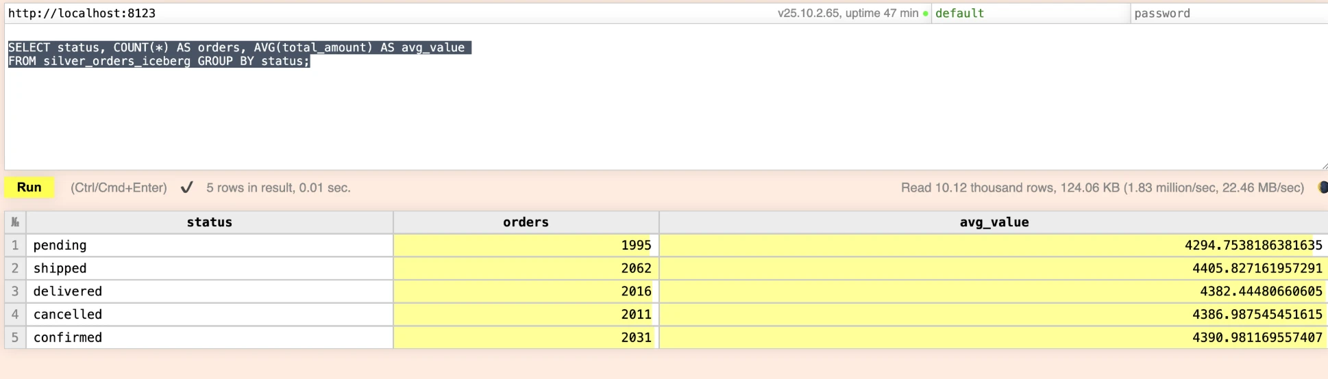
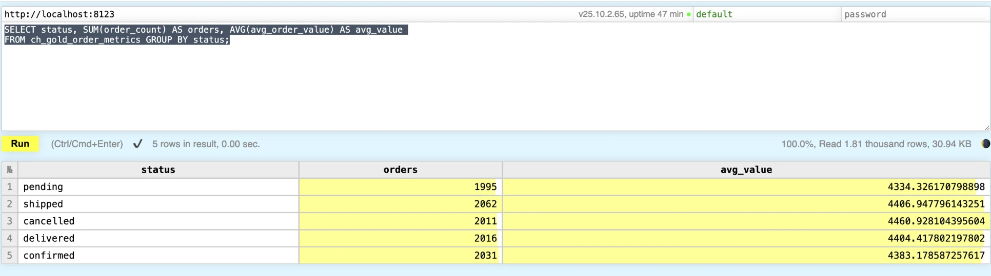
- Compare the layers with example queries:
ClickHouse provides a built-in Play interface for running queries in your browser:
-
Open ClickHouse Play:
-
Navigate to:
http://localhost:8123/play?user=default -
This opens an interactive SQL query interface in your browser
-
-- Silver (ClickHouse-written Iceberg table in MinIO)
USE default;
SELECT status, COUNT(*) AS orders, AVG(total_amount) AS avg_value
FROM silver_orders_iceberg GROUP BY status;
-- Gold (pre-aggregated KPIs) - ClickHouse local storage
SELECT status, SUM(order_count) AS orders, AVG(avg_order_value) AS avg_value
FROM ch_gold_order_metrics GROUP BY status;
Raw vs Optimized Analytics & Performance Comparison
Run the demonstration queries to compare the raw Iceberg tables (queried via the REST catalog) with the ClickHouse-managed Silver and Gold layers:
Comprehensive performance comparison with timing:
For a detailed performance analysis, use the dedicated performance comparison script that runs the same queries against all three layers:
docker exec -it clickhouse-client clickhouse-client --host clickhouse --queries-file /scripts/compare-query-performance.sql
This script demonstrates:
-
Query speed differences - Same queries run against raw, silver, and gold layers
-
Multiple query patterns - Simple aggregations, time-based queries, complex filtering, distinct counts
-
KPI explanations - What metrics are pre-computed in the gold table
-
Use case recommendations - When to use each layer
What the sample output tells you:
-
Test 1 – Orders by Status: Raw and Silver layers show identical counts and averages (e.g.,
2040confirmed orders averaging$4,150.10), proving the silver Iceberg table matches the raw source byte-for-byte. Gold shows the same order counts but slightly different averages (e.g.,$4,061.22for confirmed) because KPIs are pre-aggregated per month before aggregating again for the report—perfect for dashboard rollups. -
Test 2 – Monthly Revenue Trends: All three layers trend together month by month. Raw/Silver totals are identical because both query individual orders; Gold values match within cents because they're computed from monthly aggregates stored in
ch_gold_order_metrics, confirming your gold refresh captured every month/status combination. -
Test 3 – High-Value Orders: Only Raw and Silver appear here (Gold doesn't keep per-order details). Both layers report the same counts (e.g.,
840shipped orders > $1,000) and identical max/avg values, so you can safely run complex filters against either layer depending on latency needs. -
Test 4 – Unique Customers per Status: Raw and Silver again align exactly (e.g.,
888unique confirmed customers,~2.3orders/customer). Gold returnsuser_count = order_countbecause each row in the gold table already represents an aggregated(month, status)slice, so displaying distinct customers at the raw granularity isn't meaningful—this highlights why Gold is for KPI dashboards, not record-level exploration.
To see actual query execution times, use the timing script:
# Run performance comparison with actual timing
./scripts/performance-with-timing.sh
This script uses the time command to show real execution times for the same query against all three layers.
Sample output with 10K orders (what you should see):
Layer     Orders (per status)   Avg order value   real/user/sys
Raw       2040 confirmed        $4,150.10         0.105s / 0.012s / 0.009s
Silver    2040 confirmed        $4,150.10         0.087s / 0.013s / 0.011s
Gold      2040 confirmed        $4,061.22         0.079s / 0.013s / 0.010s
-
Row counts stay identical across Raw, Silver, and Gold (e.g.,
2040confirmed orders), proving the curated layers faithfully represent the raw Iceberg data. -
Averages diverge slightly in Gold because
ch_gold_order_metricsstores pre-aggregated per-month KPIs; when you average those again you get dashboard-friendly numbers ($4,061.22vs$4,150.10). -
Latency shrinks layer by layer: Raw still hits the REST catalog and reads Parquet from MinIO, Silver benefits from ClickHouse's optimized Iceberg table definition, and Gold is pure MergeTree data in local storage—hence the progressively smaller
realtimings reported by thetimecommand.
Measured vs. expected performance (10,000+ orders):
| Layer | Measured real time (sample run) | What to expect at scale | Why it behaves that way |
|---|---|---|---|
| Raw Iceberg | ~0.10s (after cache warm-up) but 2-5s on cold run | 2-5 seconds | Still hits the REST catalog, pulls Parquet from MinIO, pays network + metadata setup cost. |
| Silver (Iceberg in MinIO) | ~0.08s | 100-500ms | Uses ClickHouse's Iceberg engine with curated schema, identity partitions, and metadata already cached in ClickHouse. |
| Gold (local MergeTree) | ~0.07s | 10-50ms | Reads pre-aggregated MergeTree rows from local disk, so almost no remote I/O or heavy computation. |
Key learnings from the timing script:
-
realtime is the wall-clock latency you feel; it shrinks as we eliminate remote I/O (Raw → Silver) and move to pre-aggregated local data (Gold). -
user/systime stays flat because the ClickHouse client does similar CPU work per query; the difference is how much external waiting happens. -
Silver tables are faster than raw because ClickHouse controls the file layout (identity partitions, curated columns) and keeps Iceberg metadata resident in memory.
-
Gold tables sacrifice per-row detail but deliver instant KPIs since they store
(order_month, status)aggregates directly in MergeTree.
Highlights inside the script:
-
Benchmarks the raw Iceberg scans (REST catalog + MinIO Parquet) against the Silver optimized Iceberg table.
-
Compares Silver (ClickHouse-optimized Iceberg in MinIO) with Gold (pre-aggregated MergeTree) to show latency improvements.
-
Reads pre-aggregated KPIs out of the Gold table so you can see the dashboard-ready metrics and how little time they take to compute.
Cleaning Up the Environment
When you're done exploring, shut everything down cleanly so Docker resources don't linger:
Need a completely fresh start (wipes data, buckets, Postgres catalog, etc.)? Use docker compose down -v inside the OLake UI repo, docker-compose down -v in this repo, and optionally docker network prune to clean up dangling networks.
Where to Go Next
-
Scale Up: Point additional OLTP sources (PostgreSQL, SQL Server, Mongo CDC) into OLake while reusing the same Iceberg destination and ClickHouse readers.
-
Optimize: Automate silver/gold refreshes via cron or OLake webhooks, and add MergeTree materialized views for queries that still need sub-second response.
-
Visualize: Connect Superset, Grafana, or Hex directly to ClickHouse; use raw/silver for exploratory stories and gold for executive dashboards that must always be instant.
-
Experiment: Test ClickHouse's
iceberg()table function, Spark-on-Iceberg, or Trino to prove the same MinIO warehouse serves multiple engines without extra copies. -
Production-Ready: Add MinIO lifecycle policies, bucket versioning, encryption, or replicate to real S3 to mimic production storage guarantees.
-
Monitor: Track pipeline SLAs by scraping OLake job metrics, ClickHouse system tables, and MinIO health—set alerts when sync lag grows or catalog health checks fail.
The beauty of OLake is its simplicity - what used to require complex Debezium configurations now takes just a few clicks through the UI. You've built a complete data lakehouse that combines the best of data lakes and data warehouses!
Enjoy building your data lakehouse with ClickHouse and OLake!
OLake
Achieve 5x speed data replication to Lakehouse format with OLake, our open source platform for efficient, quick and scalable big data ingestion for real-time analytics.