Hilbert vs Z-order Clustering in Apache Iceberg 1.12
18 min read
Overview
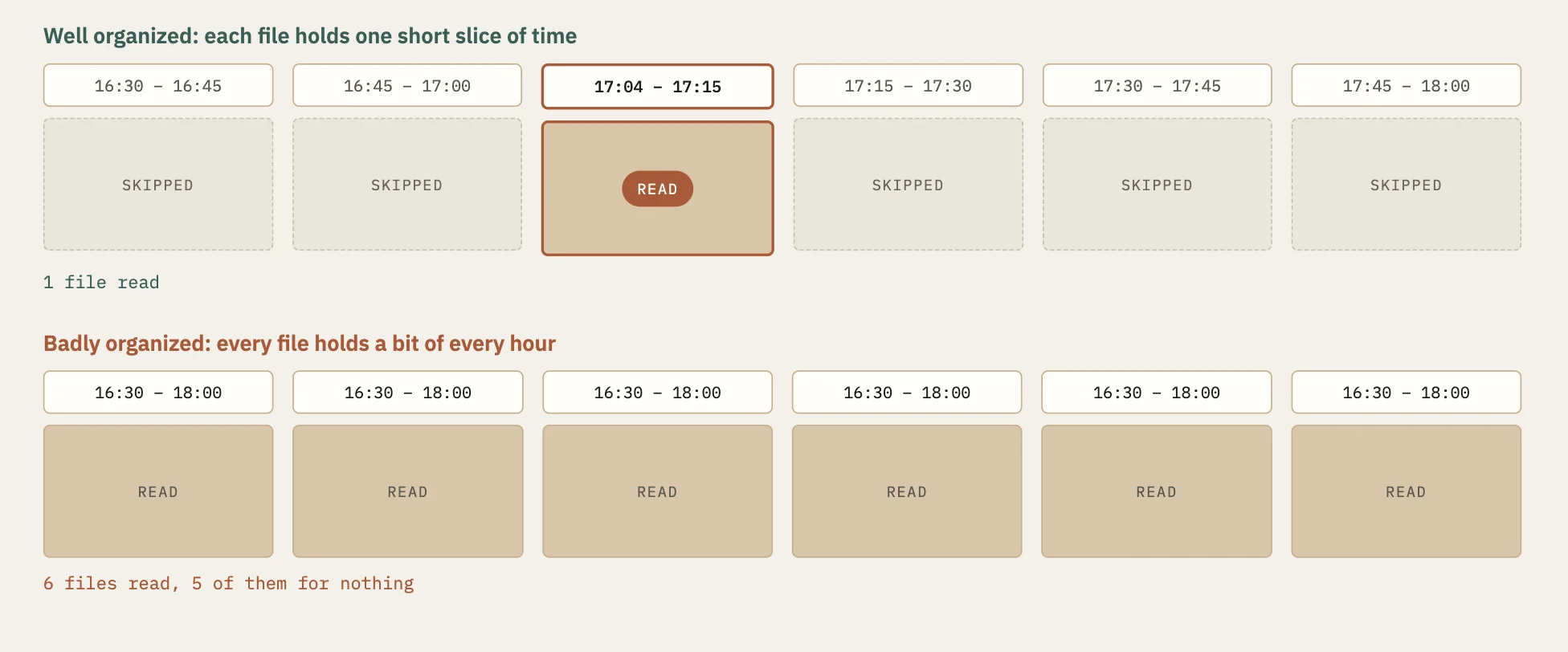
Imagine a warehouse with thousands of cardboard boxes. Each box has a label listing what's inside, such as "orders from March 3 to March 9" or "customer IDs 10,000 to 12,500." When someone asks for a specific order, the worker doesn't open every box. They read the labels and open only the boxes whose range could contain it.
A query engine reads an Apache Iceberg table in a very similar way. The boxes are the data files, and the labels are the minimum and maximum values Iceberg records for each column in each file. When every file has a narrow label, an engine can rule out most files without opening them. When the labels are wide, almost every file looks like it might hold the answer, and the engine ends up opening all of them.
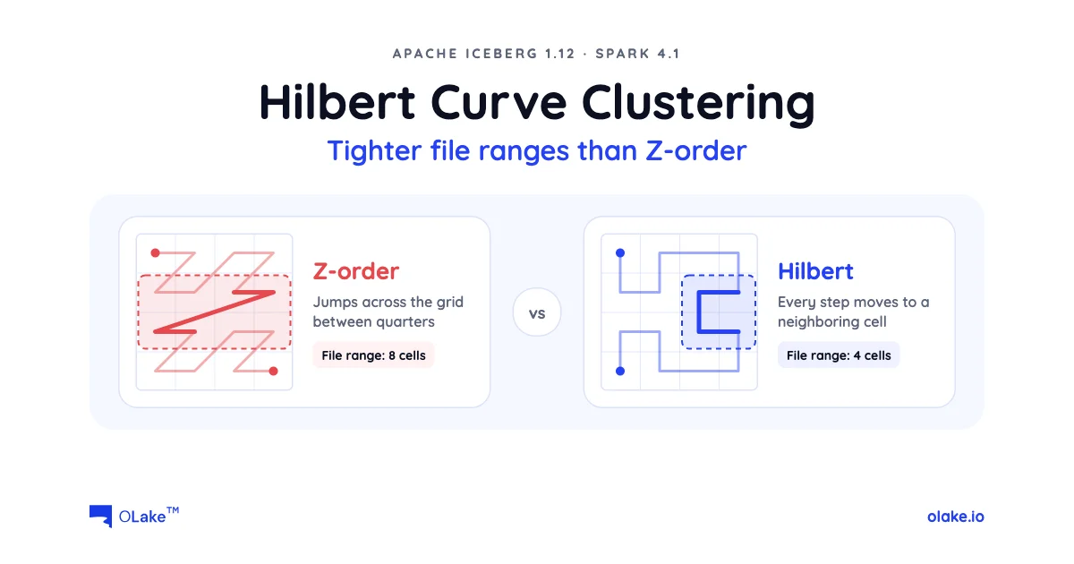
How narrow those labels are depends on how rows are grouped into files, which is what clustering controls. Apache Iceberg 1.12 adds a new way to cluster on several columns at once: the Hilbert curve, next to the Z-order curve Iceberg already had.
At OLake, we help teams move operational databases into Apache Iceberg, and keeping those tables fast to query is part of the job.
This post covers:
- what clustering is and why it decides how many files a query reads,
- the types of clustering Iceberg supports,
- where Z-order falls short,
- how the Hilbert curve fixes that,
- and how to choose between them, with the Spark commands to run each one.
What is clustering?
How Iceberg decides which files to skip
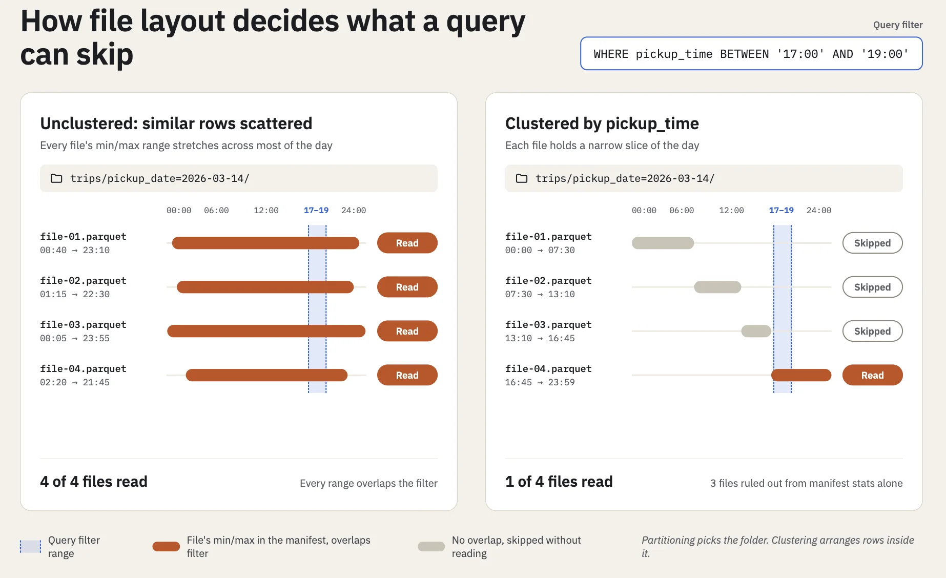
Every Iceberg table keeps a set of metadata files called manifests. For each data file, the manifest records statistics such as the lowest and highest value of each column. When a query arrives with a filter like pickup_time BETWEEN '2026-11-06 17:00:00' AND '2026-11-06 19:00:00', the engine checks each file's recorded range for pickup_time.
If a file's range doesn't overlap the filter's range at all, the file is skipped without being read. This is called data skipping.
Clustering puts similar rows in the same files
Data skipping only works as well as the rows are arranged. If rows with similar values end up in the same files, each file's range is narrow and easy to rule out. If similar rows are scattered everywhere, every file's range stretches across almost all possible values, and nothing gets skipped.
Clustering is the step that arranges the rows. In Iceberg, it happens when the data files are rewritten during compaction, by sorting the rows before they are written out.
Partitioning works at a broader level. It splits the table into folders, for example one folder per pickup date. Clustering decides which rows go into the same files inside each folder.
Types of clustering
Sorting on one column
The simplest way to cluster is a plain sort on one column. It works very well when queries filter on that one column. Many production queries, however, filter on more than one column at a time.
Consider a ride-sharing company with a trips table of a few hundred million rows. Analysts constantly filter on three columns: pickup_latitude, pickup_longitude, and pickup_time. A typical question is: show every trip that started in downtown Toronto between 5 PM and 7 PM last Friday. That's three range filters at once, one on latitude, one on longitude, and one on time.
If the table is sorted on pickup_time, the engine can skip every file outside Friday evening. But each file in that window mixes trips from the airport, the suburbs, and downtown, so its latitude and longitude ranges cover almost the whole city, and the location filters can't skip anything.
Sorting on pickup_latitude just flips the problem. Location filtering gets better, but each file now mixes trips from every hour of every day, so the time filter stops helping.
The trips table needs a way to keep rows together when they're close on all three columns at once. Space-filling curves do exactly that.
Space-filling curves: one route through every cell
Divide the city into a grid, where each cell is a small neighborhood. Now draw one walking route that passes through every cell exactly once, and number the cells in the order you visit them.
This numbering turns a two-dimensional map into a one-dimensional list, which is exactly what a sort needs. Sort the rows by their cell number, write the files in that order, and each file ends up holding one stretch of the route.
The goal is a route that stays in one part of the city for long stretches, so each file covers a small area and its latitude and longitude ranges stay narrow. The same idea works with more columns. Add pickup_time, and the grid becomes a cube, but the goal is unchanged: trips that started close together at around the same time should get nearby numbers and land in the same file.
Iceberg offers two ways to plan that route: Z-order, which it has had for several releases, and Hilbert, which is new in 1.12.
Z-order: how it numbers the cells
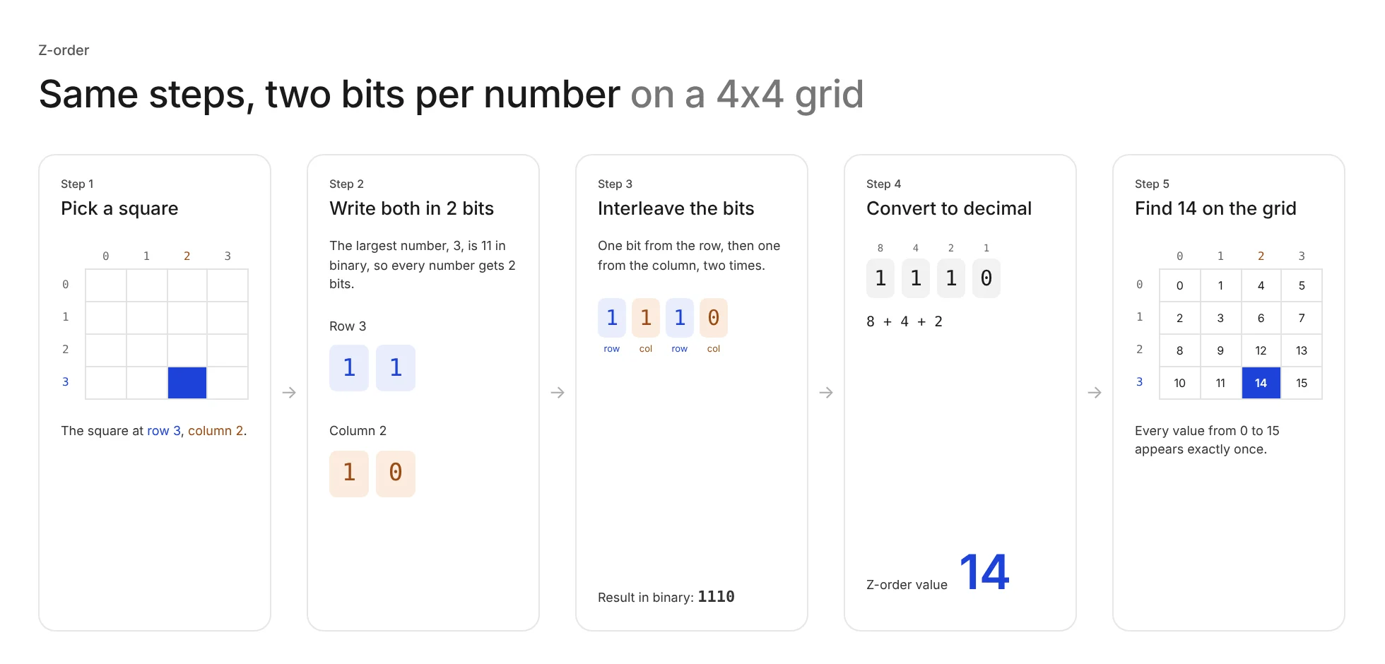
Z-order gives each cell a number by interleaving the bits of its row and column, taking one bit from each in turn.
Here's how it works on a 4x4 grid, where rows and columns are numbered 0 to 3. Take row 3, column 2 as an example.
Step 1: Write both numbers in binary.
Row 3     →  11
Column 2  →  10
Step 2: Interleave the bits. Take one bit from the row, then one from the column, and repeat until all bits are used:
first bit of row:      1
first bit of column:   1
second bit of row:     1
second bit of column:  0
together, these form the binary number 1110
Step 3: Convert it to decimal. 1110 is 8 + 4 + 2 + 0 = 14.
So the cell at row 3, column 2 gets the Z-order value 14. The process also works in reverse: split 1110 back into alternating bits, 11 and 10, and you get row 3, column 2 again.
Do this for all 16 cells, and you get this grid:
| col 0 | col 1 | col 2 | col 3 | |
|---|---|---|---|---|
| row 0 | 0 | 1 | 4 | 5 |
| row 1 | 2 | 3 | 6 | 7 |
| row 2 | 8 | 9 | 12 | 13 |
| row 3 | 10 | 11 | 14 | 15 |
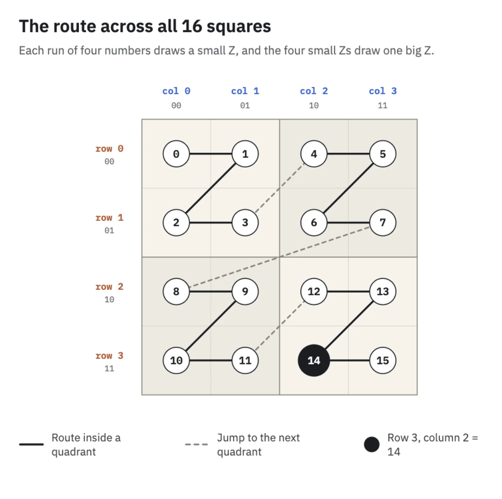
Follow the numbers 0 to 3, and they draw a small "Z" in the top-left corner. Numbers 4 to 7 draw another Z in the top-right, 8 to 11 in the bottom-left, and 12 to 15 in the bottom-right. Together, the four small Zs make one big Z, and on larger grids the same pattern repeats at every size.
The problem with Z-order
Z-order jumps between distant cells
Look at the step from 7 to 8. Cell 7 sits at the far right of row 1, and cell 8 sits at the far left of row 2. Their numbers are right next to each other, but on the map they're at opposite ends of the grid.
It's like a delivery driver who finishes a stop on the east side of town and then drives all the way to the west side for the next one, passing streets that will need a visit later anyway. The same kind of jump happens at every boundary between the Zs, and on a real table with millions of cells these jumps occur at every scale.
Why a jump widens a file's range
A jump on its own is harmless. It becomes a problem when a data file starts before a jump and ends after it, because then the file holds rows from two distant areas and its min and max range stretches to cover both.
Suppose a data file holds the rows for cells 6, 7, 8, and 9. In the Z-order grid, cells 6 and 7 sit at the right end of row 1, while 8 and 9 sit at the left end of row 2. The file's range becomes rows 1 to 2 and columns 0 to 3, which covers 8 cells even though the file only holds 4.
Now picture a query that asks for anything in column 0. This file has to be opened, because its range includes column 0, even though none of its rows are there. Multiply that by thousands of files and three filtered columns, and the wasted reads add up.
How the Hilbert curve solves this
Every step goes to a neighbor
The Hilbert curve numbers the same grid with a different route, one that never jumps. Every step moves to a cell that shares an edge with the previous one.
| col 0 | col 1 | col 2 | col 3 | |
|---|---|---|---|---|
| row 0 | 0 | 3 | 4 | 5 |
| row 1 | 1 | 2 | 7 | 6 |
| row 2 | 14 | 13 | 8 | 9 |
| row 3 | 15 | 12 | 11 | 10 |
Follow the numbers from 0 to 15, and each one is directly above, below, left, or right of the one before it.
How Hilbert builds its numbers
Hilbert uses the same binary row and column numbers as Z-order, but it reads them one pair of bits at a time, from the largest blocks of the grid down to single cells. Each pair picks one quarter of the current block.
The quarter order. Quarters are visited in a U shape: top-left is 0, top-right is 1, bottom-right is 2, and bottom-left is 3. For a row bit r and a column bit c, the quarter number is q = 2 × r + (r XOR c), and the running total grows as H = 4 × H + q.
The adjustment. Before the next pair of bits is read, the remaining bits are adjusted based on the quarter just picked. This rotates or mirrors the U inside that quarter so it starts right next to where the previous quarter ended:
- Quarter 0 (top-left): the row and column bits swap places.
- Quarters 1 and 2 (top-right and bottom-right): the bits are read as they are.
- Quarter 3 (bottom-left): the bits swap places and each bit flips, so 0 becomes 1 and 1 becomes 0.
Example 1: row 3 (binary 11), column 2 (binary 10).
- The first bits are row 1 and column 1, which point to the bottom-right quarter:
q = 2 × 1 + (1 XOR 1) = 2, soH = 4 × 0 + 2 = 2. This is quarter 2, so no adjustment is needed. - The second bits are row 1 and column 0, which point to the bottom-left cell inside that quarter:
q = 2 × 1 + (1 XOR 0) = 3, soH = 4 × 2 + 3 = 11.
The cell gets the Hilbert value 11, where Z-order gave it 14. The grid above shows 11 at row 3, column 2.
Example 2: row 1 (binary 01), column 0 (binary 00).
- The first bits are row 0 and column 0, which point to the top-left quarter:
q = 2 × 0 + (0 XOR 0) = 0, soH = 0. This is quarter 0, so the remaining bits swap: row bit 1 and column bit 0 become row bit 0 and column bit 1. - The swapped bits give
q = 2 × 0 + (0 XOR 1) = 1, soH = 4 × 0 + 1 = 1.
Without the swap, the formula would give 3, but the grid shows 1 at row 1, column 0. The adjustment is what keeps the route connected: in the top-left quarter, the U runs down, right, and back up, ending at row 0, column 1, right beside where the top-right quarter starts. In the bottom-left quarter, the U starts at row 3, column 1, right beside where the bottom-right quarter ended at row 3, column 2.
Z-order reads every block with the same Z pattern. Hilbert has to track these rotations and flips at every level of the grid, which is why it costs more CPU to compute.
Same file, tighter range
Go back to the file holding cells 6, 7, 8, and 9. With Hilbert, all four sit together in one 2x2 block.
| File's range | Cells covered by the range | Cells actually in the file | |
|---|---|---|---|
| Z-order | Rows 1 to 2, columns 0 to 3 | 8 | 4 |
| Hilbert | Rows 1 to 2, columns 2 to 3 | 4 | 4 |
For the query on column 0, the Z-ordered file has to be opened, while the Hilbert-ordered file is skipped.
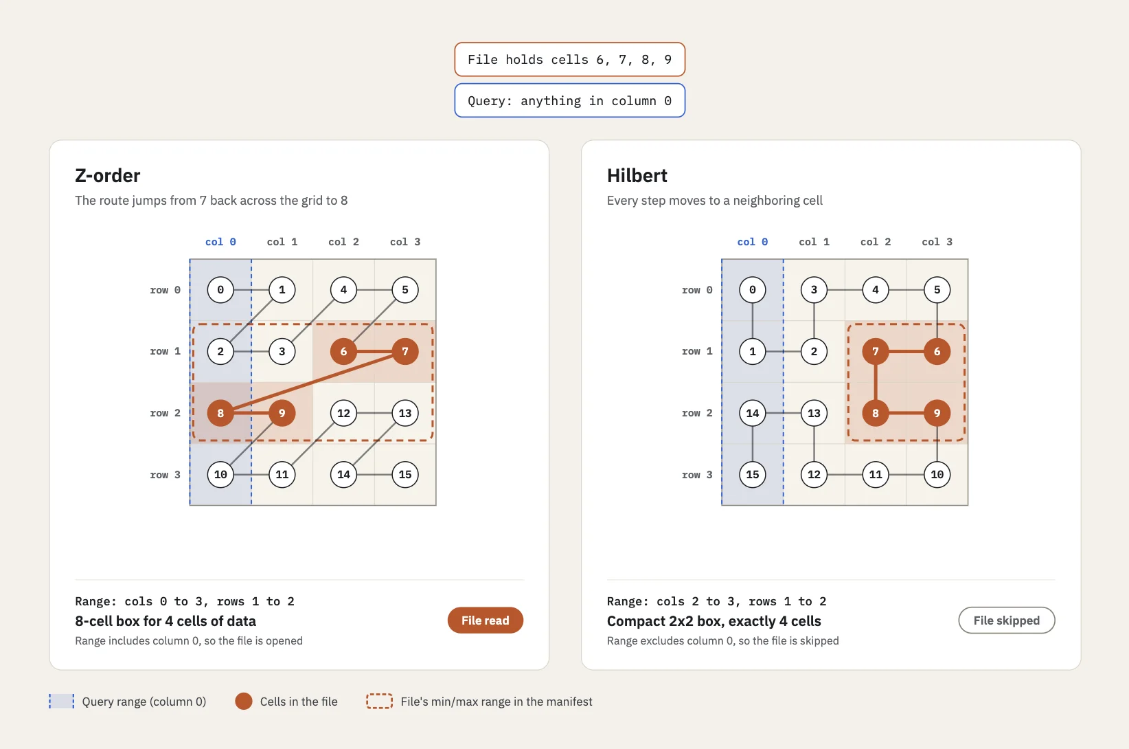
Because every step is a short one, any continuous stretch of Hilbert numbers covers one connected area of the grid rather than scattered pieces. A data file holds exactly that kind of continuous stretch, so files clustered along a Hilbert curve tend to have tighter ranges on every clustered column.
To be fair to Z-order, the two curves give the same range when a file lines up exactly with one of the quarters, such as a file holding cells 0 to 3. Real files hold whatever number of rows fits the target file size, so their boundaries rarely line up that neatly, and that is where Hilbert helps.
What Hilbert doesn't fix
Neighbors on the curve are always neighbors on the grid, but not the other way around. In the Hilbert grid, cell 2 (row 1, column 1) and cell 13 (row 2, column 1) are directly on top of each other, yet they're 11 steps apart on the route. Every space-filling curve has seams like this, because a single line can't keep every pair of neighbors close. Hilbert removes the jumps, but not the seams.
Clustering on several columns has a cost on single-column filters. This applies to both curves. When a table is clustered on d columns and written into N files, a narrow filter on just one of those columns still reads about N^((d-1)/d) files. On the trips table, clustered on three columns and written into 1,000 files, each column is split into about 10 slices. A filter on one evening of pickup_time falls into one slice and still reads about 100 files. A wider time range covers more slices and reads more. That's far fewer than 1,000, but a plain sort on pickup_time would read fewer still.
Hilbert costs more to compute. Z-order only rearranges bits. Hilbert tracks rotations and flips at every level, and that work grows with the number of columns and the precision of the curve. Clustering happens during periodic compaction rather than on every query, so the extra CPU is usually a reasonable trade, but it will show up in compaction job times.
What you should choose
Z-order and Hilbert side by side
| Z-order | Hilbert | |
|---|---|---|
| How the order is built | Interleaves the bits of each column | Recursive subdivision with rotations and flips |
| Consecutive positions | Can jump across the grid at block boundaries | Always neighboring cells |
| File ranges | Can widen when a file spans a jump | Usually tighter |
| Compute cost | Low | Higher, grows with column count |
| Best fit | Multi-column filters when compute is tight | Range filters on related dimensions such as location and time |
| Availability in Iceberg | Existing releases | 1.12, Spark 4.1 only |
Sources: Iceberg Spark procedures, apache/iceberg PR #16827 (checked Nov 2026).
A quick decision guide
Start with the queries rather than the curves.
- One column appears in almost every filter. Use a plain sort order on that column. It's the cheapest option and gives the tightest ranges on that column.
- Two or more columns appear together with roughly equal weight, and they behave like coordinates (latitude and longitude, or location and time). Try Hilbert first.
- Several columns matter, but compaction runs very often or compute is tight. Z-order is still a good default.
- The cluster isn't on Spark 4.1 yet. Z-order is the only curve available for now.
Whichever curve you choose, keep the column list short. Each column added to the clustering key weakens the locality of the others, so include only the columns that actually appear together in real filters. Clustering on six columns because they "might" be filtered on usually gives weaker results than clustering on the two that always are.
How to run Hilbert clustering in Spark
Hilbert clustering uses the same rewrite_data_files procedure as Z-order, as a sort strategy with a hilbert(...) sort order listing the columns to cluster on. For the trips table:
CALL catalog_name.system.rewrite_data_files(
  table => 'db.trips',
  strategy => 'sort',
  sort_order => 'hilbert(pickup_latitude, pickup_longitude, pickup_time)'
);
The Z-order version of the same job changes only one line:
CALL catalog_name.system.rewrite_data_files(
  table => 'db.trips',
  strategy => 'sort',
  sort_order => 'zorder(pickup_latitude, pickup_longitude, pickup_time)'
);
Before scheduling it, keep these points in mind:
- Spark version. In Iceberg 1.12, Hilbert ordering for compaction is implemented only for Spark 4.1, according to the pull request that added it. Clusters on Spark 3.5 or 4.0 need to upgrade or keep using Z-order.
- No table format change. Like Z-order, Hilbert is a compaction strategy that runs in the engine and isn't stored in table metadata, so it doesn't change the table format or its version. Any engine that reads the table afterward, whether Trino, Flink, or something else, simply sees better-organized files.
- New data isn't clustered automatically. Because the ordering belongs to the compaction job rather than the table, rows written after the rewrite arrive in their usual order. Clustering is something to schedule, not a one-time setting. Many teams limit each run to recent data with the procedure's
whereargument, for examplewhere => "pickup_time >= '2026-11-01 00:00:00'", so the job stays small. - Which files get rewritten. By default, the procedure uses the same rules as bin-pack compaction to pick files, which mostly targets small or poorly sized files. To recluster an entire table, such as when switching from Z-order to Hilbert, add
options => map('rewrite-all', 'true'), and plan for the cost of rewriting everything.
Test both on your own tables
When the right choice isn't obvious, a small experiment settles it. Dremio's Iceberg 1.12 guide gives similar advice: benchmark with your actual filter combinations, and weigh the rewrite cost along with the scan savings. A simple way to do that:
- Make two copies of a representative slice of the table, for example one month of data, using
CREATE TABLE ... AS SELECT. - Cluster one copy with Z-order and the other with Hilbert, using the same columns and target file size.
- Pick five to ten real queries from the query history, especially the slow ones that filter on the clustered columns.
- Run each query against both copies and record the number of data files scanned, not just the run time. Files scanned is what the curve directly affects, while run time also depends on cluster load and caching. The Spark UI and Iceberg's scan metrics both show how many files a query read.
- Record how long each compaction job took, since Hilbert's extra compute cost is part of the decision.
If Hilbert scans noticeably fewer files on the queries that matter, and its compaction time fits the maintenance window, switch over. If the difference is small, Z-order's lower cost may make it the better choice.
Conclusion
Clustering decides how many files a query can skip, and when queries filter on several columns together, a space-filling curve is the way to cluster. Apache Iceberg 1.12 adds the Hilbert curve next to Z-order. Because its route never jumps, it keeps related rows closer together and gives tighter file ranges.
That benefit comes with a higher compute cost during compaction, and for now it needs Spark 4.1. Z-order still has a clear place where compaction runs often or an upgrade isn't possible yet.
The right choice depends less on the curves and more on how a table is queried. The most reliable way to decide is to cluster a representative slice both ways, compare how many files each query scans, and weigh that against how long each compaction job takes.