What Makes OLake Fast? | High-Throughput Data Replication


OLake is engineered for high-throughput ELT workloads, leveraging a combination of adaptive chunking strategies & parallelized execution for historical load, and change data capture (CDC) techniques to optimize data ingestion performance.
Its architectural emphasis on concurrency, intelligent partitioning, and efficient use of system resources enables it to handle large volumes of data with minimal latency. By aligning chunk generation with source tables distribution characteristics and executing data loads in parallel across multiple threads, OLake ensures optimal throughput while maintaining consistency and scalability.
To prevent overwhelming the source database, the maximum number of concurrent threads is configurable via the source.json file, enabling users to fine-tune parallelism based on workload sensitivity and infrastructure capacity.
Types of Chunking strategies supported by olake
To maximize parallelism and throughput for full/historical load of tables, OLake splits table into manageable fragments called chunks. Each chunk can be processed independently by a dedicated worker thread, enabling concurrent extraction and transformation. Chunking is central to OLake's performance model and is tailored per source system to align with its data distribution patterns and indexing structures.
OLake supports multiple chunking strategies, each optimized for a particular database engine. The strategy selection is dynamic and driver-aware—for example:
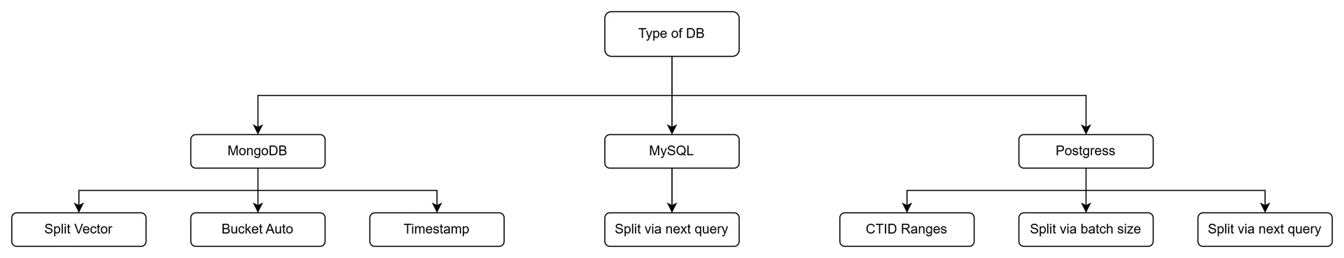
MongoDB
1. Split Vector Strategy
The Split Vector Strategy utilizes MongoDB's internal splitVector command to derive optimal chunk boundaries based on collection size and document distribution. This command is originally designed for MongoDB sharding, where it calculates split points to balance chunk sizes across shards. OLake repurposes this capability to partition data for parallel ingestion.
In this strategy, chunks are generated such that each contains approximately a fixed amount of data by default, 1024 MB per chunk. The process determines the minimum and maximum _id values in the collection and then uses splitVector to compute intermediate _id boundaries that divide the collection into chunks of roughly equal size (in MB), while ensuring no document is split across chunks.
db.adminCommand({
  splitVector: "<database>.<collection>",
  keyPattern: { _id: 1 },
  maxChunkSize: 1024
})
A key benefit of this approach is that chunking is driven by the actual data distribution, not just timestamp or primary key ranges. This improves balance across threads and avoids skewed workloads, especially in collections with irregular insert patterns.
The splitVector command is a privileged internal operation and is not permitted on MongoDB Atlas or other managed environments with restricted permissions. In such cases, OLake gracefully falls back to the bucketAutoStrategy, ensuring compatibility without user intervention
2. Bucket Auto strategy
The Bucket Auto Strategy employs MongoDB’s $bucketAuto aggregation stage to intelligently partition documents into a specified number of buckets based on the _id field.
OLake constructs an aggregation pipeline using $sort and $bucketAuto, where the number of buckets is set to 4 times the configured maximum number of threads. Each bucket returned by MongoDB contains a range (min, max) of _id values and a document count. These ranges are then used for parallel processing.
db.<collection>.aggregate([
  { $sort: { _id: 1 } },
  { $bucketAuto: {
      groupBy: "$_id",
      buckets: <MaxThreads> * 4
  }}
])
3. Timestamp strategy
The Timestamp Strategy leverages the time-encoded nature of MongoDB’s ObjectId to partition data chronologically. This is particularly effective when documents follow a time-based insertion pattern, as is common in event logs or time-series datasets.
How It Works
1. Determine Temporal Bounds:
The strategy begins by identifying the earliest and latest timestamps in the collection using the _id field’s embedded timestamp. Specifically, the first 4 bytes of an ObjectId represent the Unix time (in seconds) at which the document was created. This structure makes ObjectIds naturally increase over time, allowing them to be used as proxies for document creation time. By extracting the timestamp from the smallest and largest ObjectIds in the collection, OLake determines the temporal range of the dataset.

2. Define Time Granularity (Density):
OLake divides the total time range between the first and last record into 6 segments to estimate how data is distributed over time. Based on this, it calculates a dynamic chunk interval (density) by multiplying each segment by 10 seconds. This creates finer chunks if data is dense, and coarser chunks if it’s sparse — with a minimum granularity of 10 seconds per chunk. This approach helps balance the number of records in each chunk, even if the data insertion pattern is uneven.
timeDiff := last.Sub(first).Hours() / 6
		if timeDiff < 1 {
			timeDiff = 1
		}
density := time.Duration(timeDiff) * (10 * time.Second)
3. Generate ObjectId Boundaries:
For each interval:
-
A minimum
_idis generated by embedding the start timestamp into the first 4 bytes of theObjectId, followed by zero-padding. -
A maximum
_idis similarly generated from the end timestamp.
These ObjectIds are then used to define the lower and upper bounds of each chunk.
func generate_min_object_id(timestamp){
    """
    Generate the minimum possible MongoDB ObjectId for a given timestamp.

    Args:
        timestamp (datetime): The timestamp from which to derive the ObjectId.

    Returns:
        object_id (ObjectId): A synthetic ObjectId with the timestamp and the lowest possible suffix bytes.
    """

    # Step 1: Create a standard ObjectId from the given timestamp
    object_id = new_object_id_from_timestamp(timestamp)

    # Step 2: Overwrite the trailing bytes to make it the minimum possible value
    for i in range(4, 12):
        object_id[i] = 0x00  # Zero out all bytes after the timestamp prefix

    return object_id
}
4. Iterative Chunk Construction:
The algorithm slides the window forward by the density until it spans the entire time range. The final chunk is open-ended (Max = nil) to account for any documents inserted after the last observed timestamp.
MySql
In MySQL, OLake chunks data based on the primary key of the source table.
SELECT MIN(id) AS min_value, MAX(id) AS max_value
FROM <schema_name>.<table_name>;
To begin, OLake queries the minimum and maximum primary key values in the table. It then estimates the optimal chunk size by dividing the total row count by 8 times the number of threads configured in source.json. This 8× multiplier ensures there are more chunks than threads, allowing for better parallelism and dynamic load balancing—especially useful in cases of uneven record sizes or skewed key distributions.
func calculate_chunk_size(table_name, max_threads){
    """
    Estimate an optimal chunk size for a MySQL table to allow parallel ingestion.

    Args:
        table_name (str): Name of the source table.
        max_threads (int): Number of parallel threads configured.

    Returns:
        int: Suggested number of rows per chunk.
    """

    # Step 1: Get estimated number of rows in the table
    query = `
        SELECT TABLE_ROWS
        FROM INFORMATION_SCHEMA.TABLES
        WHERE TABLE_SCHEMA = DATABASE()
        AND TABLE_NAME = '{table_name}';
    `
    total_rows = execute_query_and_fetch_single_value(query)

    # Step 2: Divide total rows by (threads * 8) for better concurrency
    chunk_size = total_rows / (max_threads * 8)

    return chunk_size
}
The 8× multiplier used to calculate the chunk size is a design decision aimed at ensuring optimal parallelism and load balancing.
While this multiplier is based on previous performance benchmarks, it is adjustable and may be fine-tuned through further testing to match specific workloads, optimizing throughput across different environments.
Using this chunk size, OLake repeatedly executes a query to fetch the next chunk boundary using a sliding window over the primary key.
SELECT MAX(id)
FROM (
  SELECT id
  FROM <schema_name>.<table_name>
  WHERE id > start_id
  ORDER BY id ASC
  LIMIT chunkSize
) AS T;
Each chunk is defined by a Min and Max primary key value, forming a disjoint range. This range is used to split the data so each ingestion thread can process a distinct slice of the table in parallel.
# Initialize starting value
current_value = <min_value>
chunks = []

for{
    # Step 1: Build a query to find the upper bound of the current chunk
    query = `
        SELECT MAX(<split_column>) FROM (
            SELECT <split_column>
            FROM <schema_name>.<table_name>
            WHERE <split_column> > '{<current_value>}'
            ORDER BY <split_column> ASC
            LIMIT <chunk_size>
        ) AS subquery;
    `

    # Step 2: Execute the query to get the next boundary value
    next_value = execute_query_and_fetch_single_value(query)

    # Step 3: Exit loop if no more data or boundary hasn't advanced
    if next_value is None or next_value == current_value:
        break

    # Step 4: Store this chunk range
    chunks.append((current_value, next_value))

    # Step 5: Slide the window forward
    current_value = next_value
  }
# chunks now contains all (min, max) ranges for parallel ingestion
Postgresql
1. CTID Ranges
The CTID Ranges strategy is employed when a specific column for splitting the rows isn't defined. In such cases, OLake uses CTID, a system column in PostgreSQL that uniquely identifies rows within a table. This method partitions data based on relational page numbers, which represent blocks of rows in the underlying storage.
Here’s how it works:
1. Calculate the Number of Pages:
OLake starts by querying the total number of pages in the table (using PostgreSQL's relPages), which essentially represents blocks of rows stored in the table. This is done through a specialized query that counts the number of pages.
SELECT relpages
FROM pg_class
WHERE relname = '<table_name>'
  AND relnamespace = (
    SELECT oid
    FROM pg_namespace
    WHERE nspname = '<schema_name>'
);
2. Chunk Creation:
Once the total number of pages is known, the table is divided into chunks based on the batch size specified in the source.json file. Each chunk represents a set of contiguous pages, where the size of each chunk corresponds to the batch size defined by the user. For example, if the batch size is set to 100, each chunk will encompass 100 pages.
# Inputs:
# - total_pages: Total number of pages in the table (from PostgreSQL)
# - batch_size: Number of pages per chunk (from config)

for start_page := uint32(0); start_page < total_pages; start_page += batch_size {
	end_page := start_page + batchSize

	# If this is the last chunk, make it open-ended using a very large value
	if end_page >= total_pages {
		end_page = MAX_UINT32  # acts as "infinity" for CTID comparison
	}

    # Format the CTID boundaries as strings
    min_ctid = f"'({start_page},0)'"
    max_ctid = f"'({end_page},0)'"

    # Append the chunk (min, max) range
    chunks.append((min_ctid, max_ctid))
  }
3. Handling the Last Chunk:
The last chunk might not always contain a full batch of pages. To handle this, the end of the last chunk is set to the maximum possible value (^uint32(0), which is the maximum value for uint32), ensuring that the final chunk captures any remaining rows.
4. Chunk Ranges:
Each chunk is represented by a Min and Max CTID, where the CTID corresponds to the relational page range of the chunk. This allows each chunk to represent a specific section of the table based on page boundaries.
Postgres - If split column is defined
2. Split via batch size
The Split via Batch Size strategy is employed when the split column contains numeric types (integer or float), ensuring even distribution of chunks across threads for efficient processing.
1. Chunk Calculation:
The minimum and maximum values of the split column are retrieved from the dataset.
The chunk size is based on the batch size configured in the system. Each chunk represents a range of values determined by the batch size.
2. Chunk Boundaries:
Starting from the min value, the function repeatedly adds the batch size to determine the max value for the current chunk. This process continues until the maximum value of the split column is reached.
# Inputs:
# - min_value: Starting point of the first chunk
# - max_value: Upper limit of the split column
# - dynamic_chunk_size: Range size for each chunk (from config)

splits = []
chunk_start = min_value
chunk_end = chunk_start + dynamic_chunk_size

for CompareValues(chunkEnd, max) <= 0 {
	# Create the current chunk with range (chunk_start, chunk_end)
    splits.append((chunk_start, chunk_end))

	# Slide the window forward
    chunk_start = chunk_end
	chunk_end = chunk_start + dynamic_chunk_size
}
The final chunk is adjusted to include any remaining data after the last full chunk, with the max value set to nil for the last chunk.
3. Split via next query
The Split via Next Query strategy is used when the specified split column does not contain a numeric data type (e.g., integer or float). Instead, this method leverages queries to determine the boundaries for each chunk, ensuring the data is partitioned effectively even when numerical ranges are not applicable.
1. Chunk Calculation:
The column is sorted in ascending order, and boundaries for the chunks are determined through successive queries.
SELECT MAX(<column>)
FROM (
  SELECT <column_name>
  FROM "<schema_name>"."<table_name>"
  WHERE <column_name> > '<last_seen_value>'
  ORDER BY <column_name> ASC
  LIMIT <batch_size>
) AS T;
For example, if splitting on a uuid column in table users under schema public, and the last seen value was uuid-001 with a batch size of 25, the query would look like:
SELECT MAX(uuid)
FROM (
  SELECT uuid
  FROM "public"."users"
  WHERE uuid > 'uuid-001'
  ORDER BY uuid ASC
  LIMIT 25
) AS T;
For each iteration, the starting point (minimum) of the current chunk is used to query the database for the next chunk's endpoint. This process continues until no new chunks are found or the end point equals the start point, indicating that no further chunks can be generated.
2. Chunk Boundaries:
Each chunk is defined by its start value (current chunk start) and end value (determined by the query). The process is repeated, progressively moving through the data set and partitioning it into appropriately sized chunks based on the batch size.
# Inputs:
# - split_column: The column used to split (e.g. UUID, string, etc.)
# - table_name: Name of the source table
# - schema_name: Schema in which the table resides
# - chunk_size: Number of records per chunk
# - min_value: The minimum value to start from (first row’s value)

splits = []
current_value = min_value

for {
    # Step 1: Query to get the highest value in the next <chunk_size> rows after current_value
	query := `
        SELECT MAX(<split_column>) FROM (
            SELECT <split_column>
            FROM <schema_name>.<table_name>
            WHERE <split_column> > '{current_value}'
            ORDER BY <split_column> ASC
            LIMIT <chunk_size>
        ) AS subquery;
	`
	next_value = execute_query_and_fetch_single_value(query)

    # Step 2: If there's no next value, we're at the end of the data
    if not next_value or next_value == current_value:
        # Final chunk is open-ended
        splits.append((current_value, None))
        break

    # Step 3: Save the current chunk
    splits.append((current_value, next_value))

    # Step 4: Move to the next window
    current_value = next_value
}
OLake
Achieve 5x speed data replication to Lakehouse format with OLake, our open source platform for efficient, quick and scalable big data ingestion for real-time analytics.