OLake Terminologies

Streams

A Stream in OLake Go represents a unit of data (such as a table or collection) discovered from a source. This panel lets you choose which streams to sync, how the data is synced (i.e. you can choose from different sync modes), what schemas they use, and also allows the user to do partitioning on data before loading it into the destination.

Streams Properties

1. Normalization

Normalization in OLake Go is the transformation step that does Level-1 flattening of data in nested JSON format, mapping fields to proper columns, thus making data ready to be written into Iceberg/Parquet format tables.

• Detects schema evolution (adds, drops, type promotions) and writes according to Iceberg v2 spec.
• Flattens nested structures so records become query-friendly.
• Focuses on mapping source types to Iceberg/Parquet types.

For input as given below,

note

Normalization must be enabled at the schema configuration step per table or stream within the job.

Queried using AWS Athena
Initial state: Sync done, when normalization is off. Focus on the data column.

After state: Sync done, when normalization is on.

Advantages:

• Normalized streams can be queried with standard SQL—no unusual parsing or UDFs needed.
• Schema evolution (adds/drops/type promotions) is detected and written per Iceberg v2 spec, so downstream tables continue to operate without pipeline breaks as source schemas evolve.
• With transformation and normalization integrated into the pipeline (before the write) mean no extra post-processing jobs, so no extra Spark/DBT/Glue jobs later to "fix" the shape is required.

---

2. Sync Modes

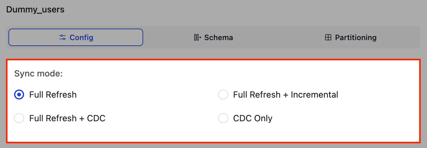
Sync modes in OLake Go define the strategy used to replicate data from a source system to a destination. Each mode represents a different approach to data synchronization, with specific behaviours, guarantees, and performance characteristics.

OLake Go supports 4 distinct sync modes:

1. Full Refresh:
   Entire table is re-copied from source to destination in parallel chunk every time the sync is run. Useful as a main sync mode or for initial loads.

2. Full Refresh + CDC (Change Data Capture):
   Real-time replication that first does a full-refresh, then streams changes (inserts, updates, deletes) in real-time.

3. Full Refresh + Incremental:
   Syncs the records by comparing a cursor field value. Starts with a full-refresh, then in subsequent syncs reads only rows where the cursor field value is greater than the last synced cursor field value. For example, if the last synced cursor field value was id = 7, the next sync reads only records with id > 7.

   How Cursor Fields Work

   A cursor field is a column used to track which records have been synced. OLake Go remembers the maximum cursor value from the previous sync and only fetches records with higher values in the next sync.

   Important: The choice of cursor field determines what changes are tracked:

   • Using auto-increment columns (like id or primary key) : Only new rows are synced. Updates or deletes to existing rows (like changing id = 7) are not tracked because their id value doesn't change.
   • Using updated_at or timestamp columns: Both new rows and updates to existing rows are synced because the updated_at value changes when a row is modified, making it behave similar to CDC. Deletes are still not tracked.

   Cursor Field Configuration:

   • Primary Cursor (required): The main column used to track sync progress (e.g., id, created_at, or updated_at).
   • Secondary Cursor (optional): Used as a fallback when the primary cursor value is null.

4. CDC Only:
   A CDC variant that skips full-refresh entirely, focusing on processing only the new changes after CDC begins.

note

Changing the sync mode triggers Clear Destination.

---

3. Data Filter

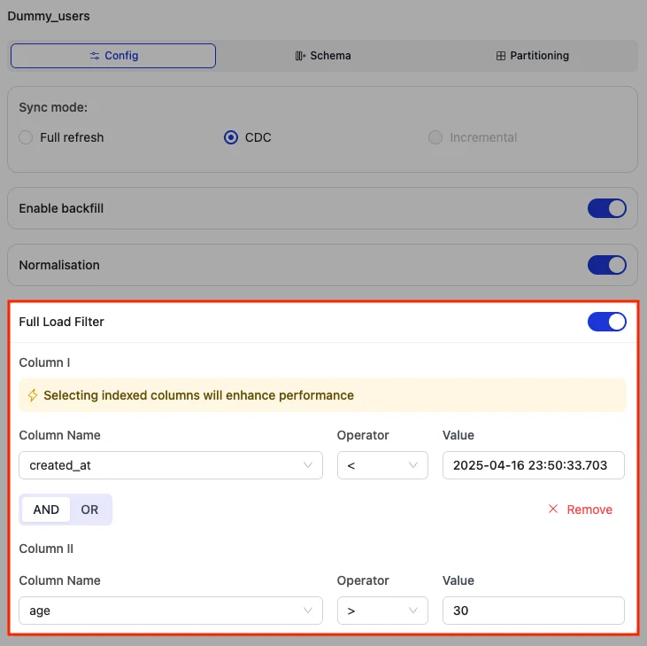
The data filter feature allows selective ingestion from source systems by applying filtering conditions before writing to the destination, so only the required subset of data is replicated.

• Ensures only selected data enters the pipeline, saving on transfer, storage, and processing.
• Supports combining up to two conditions with logical operators (AND/OR).
• Operators: >, <, =, !=, >=, <=
• Values can be numbers, quoted strings/timestamps/ids (eg.created_at > 2025-08-21 17:38:35.017), or null.

note

Data filter is supported only when Normalisation is enabled for the job.

CDC/Incremental Filter Behavior

• From OLake Go connector v0.6.0 and OLake UI v0.4.1 onward, data filter is now available for CDC and Incremental sync as well, and the filter configured during Full Refresh will be applied during subsequent CDC and Incremental syncs.
• Data filtering for CDC and Incremental is available only for jobs created on OLake Go connector v0.6.0 or later. For jobs created on earlier versions, even if a data filter is configured for Full Refresh, it will not be applied during CDC and Incremental, even if the OLake Go version is upgraded; new job must be created to use data filtering for CDC and Incremental.
• If you update an existing job’s filter after it has been created and scheduled (for example, changing conditions a few days later), OLake Go will automatically perform Clear Destination, and the next sync will run as a Full Refresh that applies the new filter conditions.
• If a job was originally created without any filter and you later add a filter, OLake Go will again perform Clear Destination, and the next sync will be a Full Refresh that uses the newly added filter.

---

4. Schema

Schema is the structure of the tables (or streams) that OLake creates when it scans and discovers the source data. The ability to adjust a schema (add/remove columns, change types) without rewriting the entire table is called Schema Evolution. For more information, refer to Schema Evolution Feature.

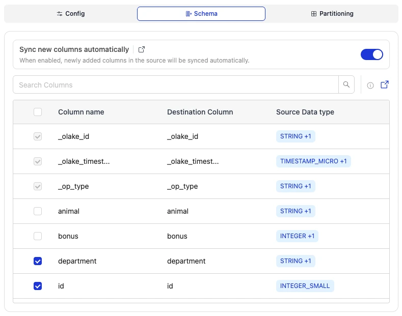
After streams discovery is complete, OLake Go presents all available columns for each selected table. Schema management in OLake Go allows you to control which columns from your source tables are synced to the destination, enabling you to evolve your schema by selecting or deselecting columns as needed.

• Column Selection:

  • By default all the columns are selected, and users can unselect any column they do not want to sync to the destination.
  • OLake Go-generated columns cannot be deselected. For more information about these columns, refer to OLake Go-Generated Columns.
  • Any modifications to column selection will take effect starting from the next sync.
  How Column Selection Impacts Existing Data

  • If a job previously had all columns selected and some columns are later deselected, the deselected columns will no longer sync new data in subsequent syncs. However, the historical data for those columns will remain in the destination.
  • When new columns are added to the source and enabled in OLake Go, they will be synced starting from the next run. Previously ingested records in the destination will not be backfilled, and the new columns will remain null (or blank) for those older rows.
  • If you want data for newly selected columns to be populated for all existing rows in the destination, you must run Clear Destination to clear all existing data in the destination and perform a full load again.

• Sync new columns automatically:
  • By default, this toggle is enabled, ensuring that any new columns added to the source are automatically selected and synced in the next sync.
  • When disabled, users must manually edit their streams and select the new columns which they want to be included in the sync.

• Source Naming Convention:

  • By default, this toggle is disabled, ensuring that column names are normalised to follow destination naming conventions before being written to the destination.

    

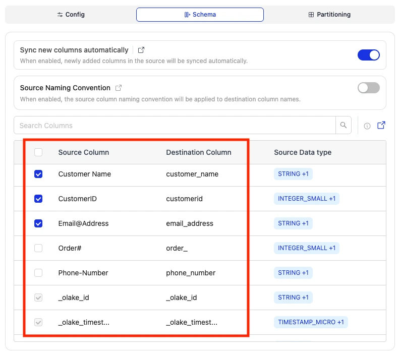
  • When enabled, column names are written to the destination exactly as they appear in the source.

    

Version Compatibility

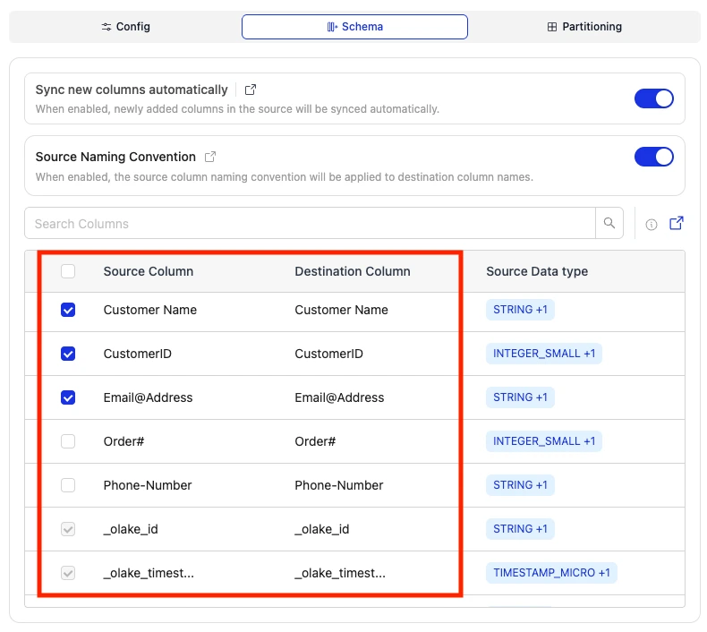
• Column selection and automatic sync of new columns are available in OLake Go v0.4.0 and OLake UI v0.3.1 or later.
  Jobs created before these versions must be run on OLake Go v0.4.0+ and OLake UI v0.3.1+ to use these features; newly created jobs have them enabled by default.
• Source Naming Convention is available in OLake Go v0.7.7 and OLake UI v0.4.7 or later.

---

5. Partitioning

Partitioning organizes data by grouping similar rows based on column values or transformations, enabling efficient query processing and data management. In simple terms, routes output by record values. The result is fewer data files scanned, less I/O, and faster queries.

info

Unlike traditional systems like Hive, Iceberg's approach uses "hidden partitioning," where partition details are managed in metadata rather than physical folders or explicit columns.

• Usage Format: "partition_regex" = "/{field_name, transform}/{next_field, transform}"
  Example:-
  • Partition Regex : "/{created_at, day}" => Partitioning done on the created_at field, transformed using 'day'.

For input as given below,

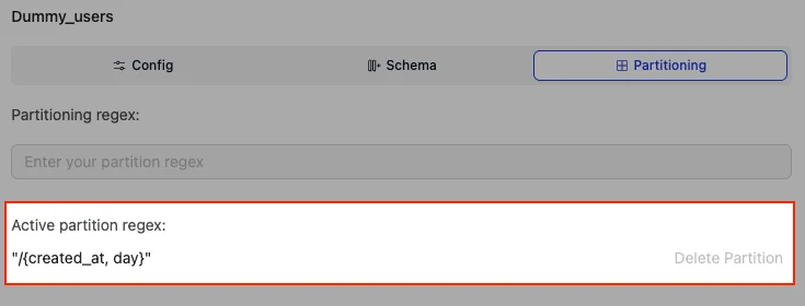
As seen below, partition on created_at field, tranformation using 'day' has been done.

Benefits of Partitioning:

• Faster Data Retrieval: Queries filtering on partitioned columns (e.g., time ranges) only scan relevant partitions, avoiding full table scans. For instance, in a logs table partitioned by date, a query for a specific day skips files from other dates, potentially speeding up results by orders of magnitude for large tables.
• Automatic Partition Pruning: In case of Iceberg, it derives partition filters from logical predicates without requiring users to add extra filters, unlike Hive where missing partition conditions lead to scanning all data. This can improve query times highly in real-world scenarios, such as financial data analysis. This feature is vital for streaming logs, e-commerce orders, or IoT telemetry etc.
• Efficient Handling of High-Volume Data: For high-cardinality fields (e.g., user IDs), transforms like bucketing distribute data evenly, preventing hotspots and enabling balanced query loads. Combined with sorting within partitions, this further optimizes scans by leveraging min/max statistics in file footers. For example, using “/{user_id, bucket[512]}", will hash user_id and assign it to buckets ranging from 0 - 511.
• Diverse Transforms: Supports flexible operations like identity, year/month/day/hour extraction, bucketing, and truncation, enabling tailored partitioning for various use cases (e.g., time-series data or categorical grouping). For example, bucketing high-cardinality keys like UUIDs into fixed groups improves write distribution and query efficiency.
• Schema Independence: Partitioning isn't tied to the table's schema, so you can evolve schemas (e.g., add columns) without breaking partitioning or queries.
• Hidden Partitioning: Writers don't need to manually compute or supply partition values; For example, Iceberg derives them from source columns (e.g., converting a timestamp to a date). This avoids silent errors like incorrect formats or time zones (common in Hive).

---

6. Table/Column Normalization & Destination Database Creation

Table/Column Normalization

Table and column names are normalized to ensure compatibility with tools like AWS Glue etc., which do not support uppercase letters or special characters. Specifically:

• Uppercase letters are converted to lowercase
• Spaces and special characters are replaced with underscores (_)

Example:

Customer Details-1 → customer_details_1

Destination Database

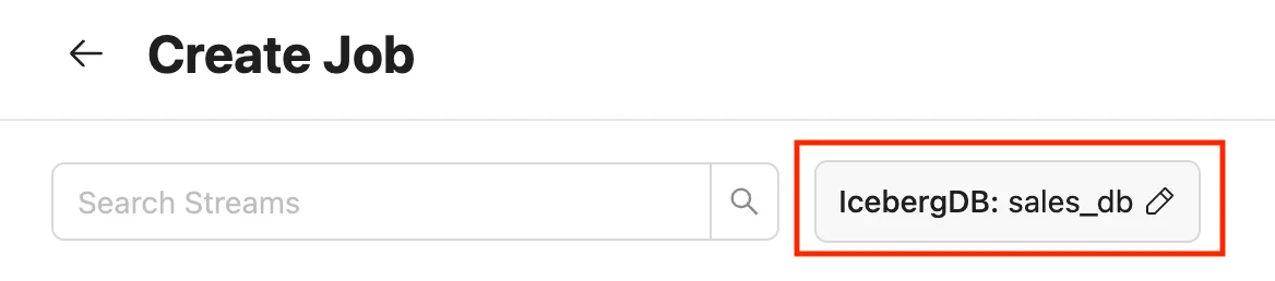
When a job is created and streams are discovered, a destination database is automatically created to store the synced tables.

The default destination database name is:
jobname_database_{$source_namespace$}

In case of sources like MySql, Oracle etc., it will be:
jobname_{$source_namespace} where source_namespace = database

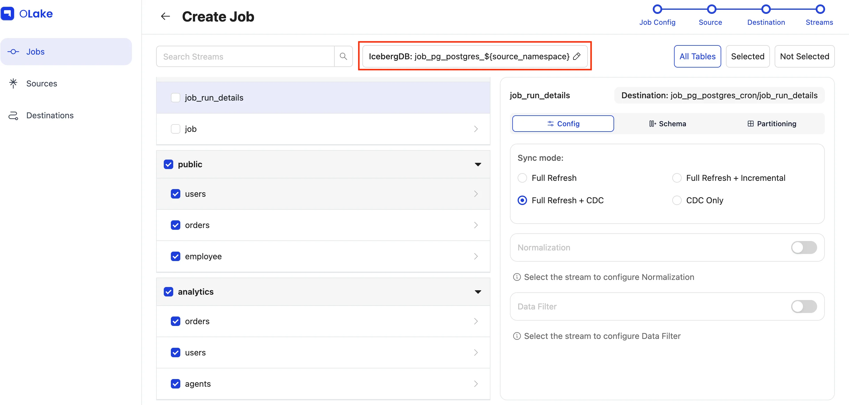
Users can rename/modify the database name by clicking the edit icon.

When editing the destination database, there are two options:

1. Dynamic (Default)

The database name prefix is set to jobname_database by default, followed by the dynamic source namespace. Users can customize the prefix to any value, which will then be applied across all namespaces. The resulting destination databases with the chosen prefix will be displayed in a list.

2. Custom

This option allows users to create a single, custom destination database for all streams, without including the namespace. As a result, all streams will share a single destination database name.

The database name will be updated here after saving the changes.

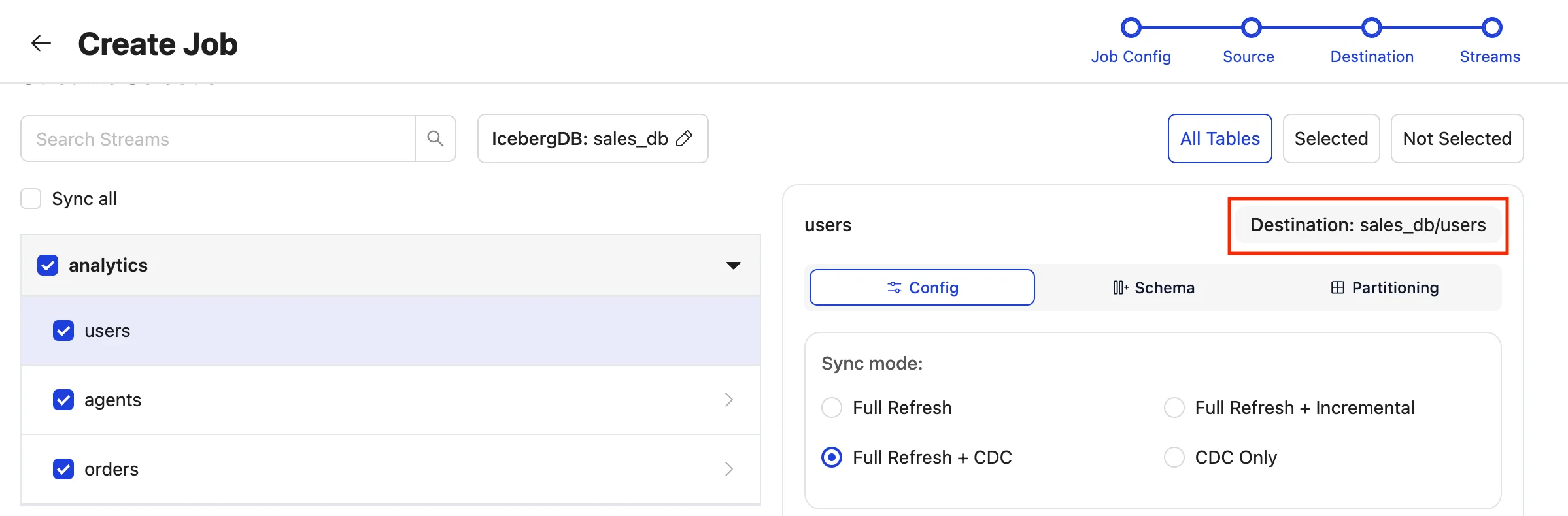
For each stream, the destination will be displayed within the stream’s configuration settings as:
destinationDB/normalised_tablename

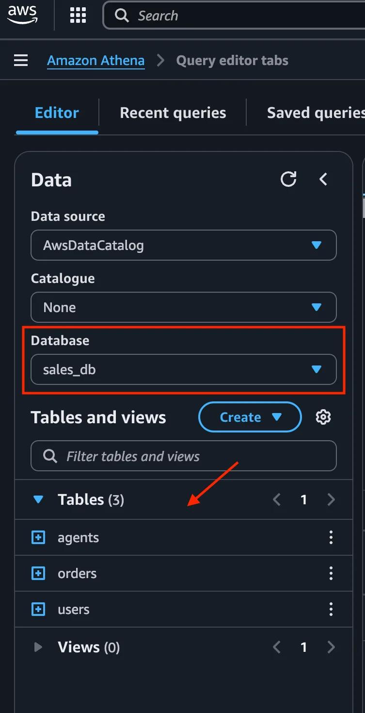
Once the sync is complete, the streams will be available in the Iceberg database at the destination, with the corresponding tables stored within it and can be queried by any query engine.

---

7. Modes to Ingest Data (Upsert vs Append)

These modes control how records are written to the destination for CDC and Incremental syncs. These modes can be configured in the Streams panel after discovery completes.

info

• By default, all streams are set to All Upsert, except for Kafka source which defaults to Append mode.
• All streams can be switched to Append with the global selector All Append, or overridden per table via the stream’s Ingestion Method.

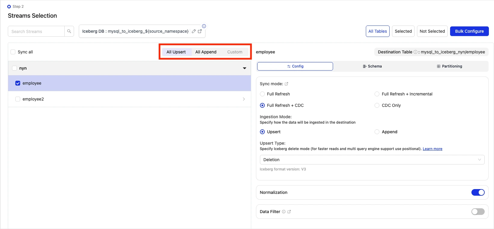
Ingestion Mode

• Available in the Streams panel for each table/collection via the stream’s Ingestion Method control.
• Use it to override the global selection (All Upsert or All Append) for specific tables.
• Example: Consider three tables— orders, customers, and logs in the Streams view. Keep the global mode as All Upsert for orders and customers to only observe the latest state, and set logs to Append in its Ingestion Method to retain full history; the global selector then shows Custom which indicates that we have a combination of append and upsert modes in the particular sync.

Important to Know!

• What happens when newly discovered streams show up in the Streams panel?
  • If all tables are Upsert (global All Upsert), new tables default to Upsert.
  • If all tables are Append (global All Append), new tables default to Append.
  • If the selection is Custom (mix of Append and Upsert), new tables default to Upsert. To change this for any table, adjust the per-table Ingestion Method in the Streams section or apply a global selection before running.
• Full Refresh is always Append. The Append/Upsert choice applies to CDC and Incremental phases.

Upsert

• Ensures no duplicate records at the destination. For a given key, only the most recent row value is transferred and kept in the destination.

• When using Upsert mode, OLake Go offers three upsert type options for writing to Iceberg destinations:

  • Equality Deletes: Identifies rows to delete by matching primary key values (Iceberg V2).
  • Positional Deletes: Identifies rows to delete by file path and row position (Iceberg V2).
  • Deletion Vectors: Identifies rows to delete using a compact bitmap per data file (Iceberg V3).

  The default delete format is determined by your selected query engine and follows this order: equality deletes, positional deletes, then deletion vectors, selecting the first format your engine supports. Different streams can have different upsert type in a particular job.

  Kafka source

  • For Kafka source, only positional deletes are supported.

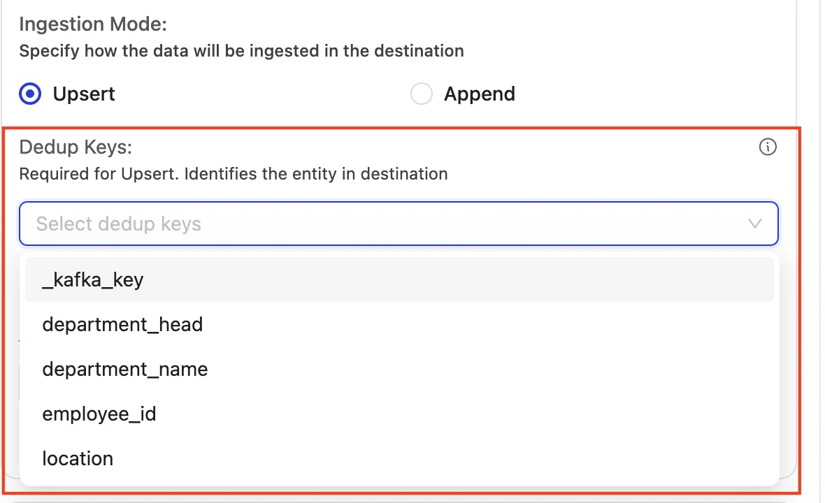
  • When Upsert is selected, you must configure at least one Dedup Key in the stream Configuration tab before the job can be saved.

    

  See Delete Format Support by Query Engine to check which formats different query engines support. The upsert functionality remains the same, only the format of delete files changes.

  Upsert Type Changes

  • Switching from equality deletes to positional deletes or deletion vectors on existing jobs is supported. Subsequent syncs use the new format, and OLake Go builds indexes to migrate existing equality delete files to the new format.
  • Switching from deletion vector to equality/positional deletes and vice versa on existing jobs will trigger clear destination operation because this is an Iceberg version downgrade (v3 to v2).
  warning

  Delete format options require every component below to meet these minimum version requirements.

  • OLake Version 0.11.0 and above.
  • OLake UI 0.6.0 and above.
  • Helm chart 0.0.28 and above.
  • OLake worker 0.3.11 and above.

  For instance, if the OLake UI is updated but the OLake worker, Helm chart, or OLake Version is still on an older version, sync jobs might fail.

  info

  Positional deletes and deletion vector need persistent index storage. To learn how to set that up for your deployment, see:

  • Kubernetes (Helm): Index Storage for Positional Delete/Deletion Vector Writes
  • Docker Compose (OLake UI): Index DB Setup for Positional Delete/Deletion Vector Writes

• Example: Suppose a transaction with id = 1 changes over time:

  1. T1: amount = 100, status = "created"
  2. T2: amount = 120, status = "closed" (latest)

  With Upsert, the destination keeps only the latest version for id = 1 (T2: amount = 120, status = "closed"). Earlier versions are not kept as separate rows.

• Equality deletes: How duplicates are avoided: A delete file is maintained that stores the _olake_id of the previous version.

  • Before change (T1 ingested): destination has id = 1 with amount = 100, status = "created".
  • On change (T2 ingested via CDC): the existing id = 1 is referenced in the delete file; the new row for id = 1 with amount = 120, status = "closed" is written to destination.
  • Result: destination retains only the latest row for id = 1 (T2), so no duplicates.

• Positional deletes: How duplicates are avoided: A positional delete file records the data file path and row position of the previous version. OLake Go maintains an index that maps each _olake_id to where its current row lives in the table.

  • Before change (T1 ingested): destination has id = 1 with amount = 100, status = "created" in a data file (for example, .../data-00001.parquet at row position 42).
  • On change (T2 ingested via CDC): the delete file marks that file path and row position as deleted; the new row for id = 1 with amount = 120, status = "closed" is written to destination.
  • Result: destination retains only the latest row for id = 1 (T2), so no duplicates.

• Deletion vectors: How duplicates are avoided: A binary bitmap (deletion vector) is maintained per data file, stored in a Puffin file, with one bit per row position. OLake Go maintains an index that maps each _olake_id to the data file and row position where its previous version lives, same as with positional deletes.

  • Before change (T1 ingested): destination has id = 1 with amount = 100, status = "created" in a data file (for example, .../data-00001.parquet at row position 42).
  • On change (T2 ingested via CDC): the bit at position 42 in the deletion vector for data-00001.parquet is set to 1 (deleted); the new row for id = 1 with amount = 120, status = "closed" is written to destination in a new data file.
  • Result: destination retains only the latest row for id = 1 (T2), so no duplicates. Readers skip position 42 by checking the bitmap instead of scanning multiple delete files.

• Recommended for transactional tables where the latest state is required (e.g., orders, customers, products).

Append

• Adds all incoming records to the destination without deduplicating. Every change event becomes a new row.
• Example: Using the same sequence for id = 1, the destination will contain both T1 and T2 as separate rows. This preserves the change history, enabling analysis of how the record evolved over time.
• Recommended for audit, logs, and event streams where full change history is desired.
• No delete files: All records are transferred to the destination as-is, even if duplicates occur.

---

8. Bulk Configure

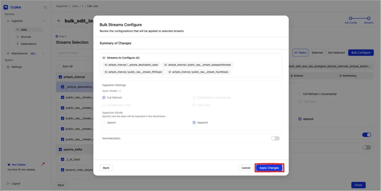
Bulk Configure lets users apply the same configuration to multiple selected streams at once. When working with sources containing multiple streams, users often need to apply the same configuration across several streams. Bulk Configuration significantly reduces setup time and improves usability.

Supported Bulk Configurations

When multiple streams are selected using checkboxes, users can trigger a bulk configuration action to apply the following properties for all selected streams at once:

• Sync Mode
• Cursor Fields: Shown only if Sync mode is Full Refresh + Incremental. Only columns that are common across all selected streams are available for cursor field selection.
• Data Filter (Column and Values): Only columns that are common across all selected streams and have similar data types are available for data filter configuration.
• Deduplication Keys (Kafka only): When Upsert mode is selected for Kafka sources, only columns that are common across all selected streams are available for dedup key selection.
• Partition Regex Value

Important Considerations

• Overwriting Existing Configurations: Existing configurations are overwritten only for the modified properties. If a user uses the bulk configure option to change only a few properties of a previously configured stream, properties configured outside the bulk configure feature remain unchanged.
• Warning on Reconfiguration: If a few streams are already configured and the user configures them again via Bulk Configuration, a warning modal will appear to confirm the action. Changing an already configured stream property will trigger a clear destination run.

Step 1: Initiate Bulk Configuration

From the Streams page, the Bulk Configure button can be used to apply the same configuration across multiple streams at once.

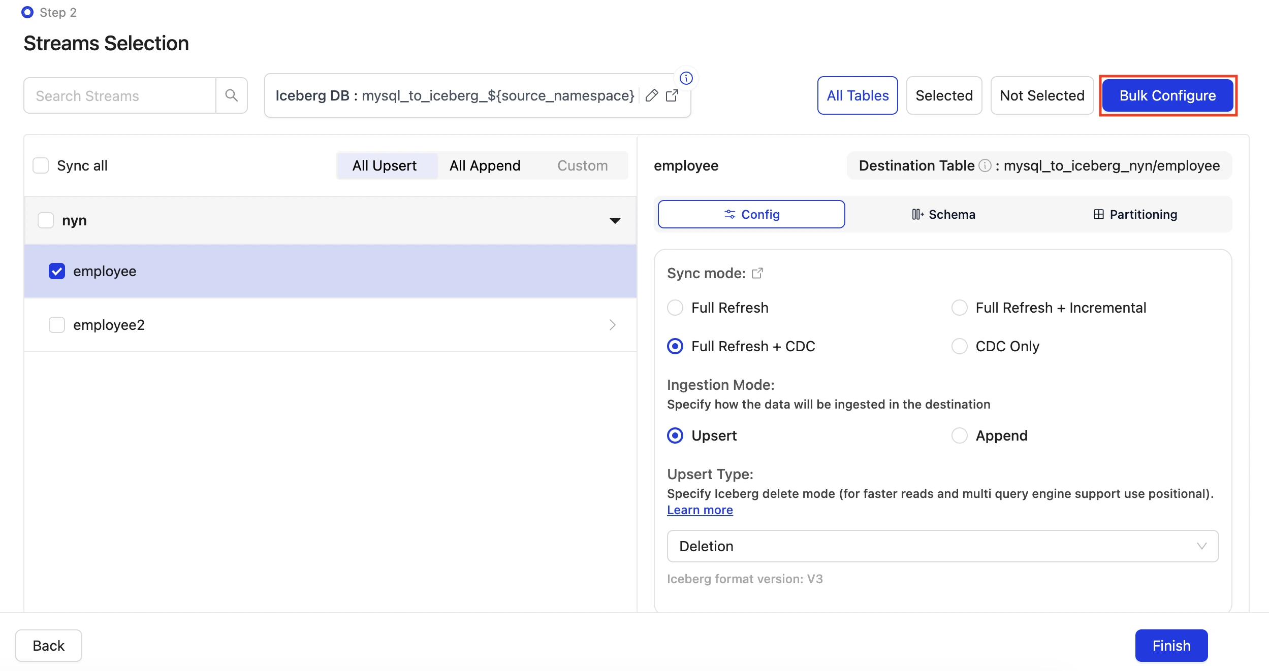
Step 2: Select Streams

After clicking Bulk Configure, a modal opens where the target streams can be selected for bulk configuration. Once stream selection is complete, click Configure Streams to continue.

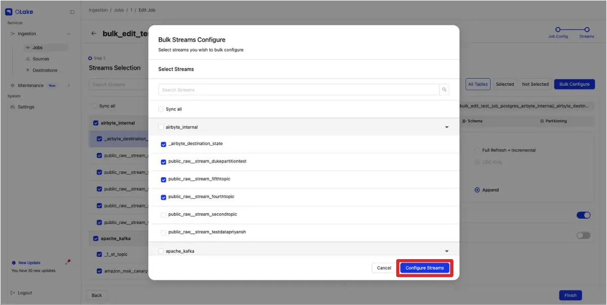
Step 3: Select Configuration

The next window displays the selected streams for bulk configuration. Configure the properties to be applied across those streams. The properties that are configured are marked with a warning sign, and only those marked properties are applied.

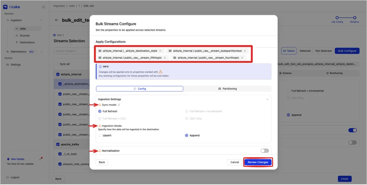
Step 4: Review and Apply Configuration

In the final window, the selected configuration can be reviewed before submission. After confirmation, clicking Apply Changes applies the configuration to the selected streams.