This blog presents an in-depth examination of modern data partitioning techniques, with a strong focus on the transition from Apache Hive's explicit, folder-based approach to Apache Iceberg's innovative metadata-driven partitioning.

The blog explores the core concepts of partitioning, outlines the limitations of legacy partitioning strategies, and explains how modern approaches have been architected to overcome the scalability and manageability challenges of large, evolving datasets. the operational and management challenges posed by massive and evolving datasets.

Introduction to Data Partitioning

Partitioning a database is the process of breaking down a massive dataset into smaller datasets and distributing these smaller datasets across multiple host machines(partitions), based on key attributes. Every host instance can hold multiple smaller datasets.

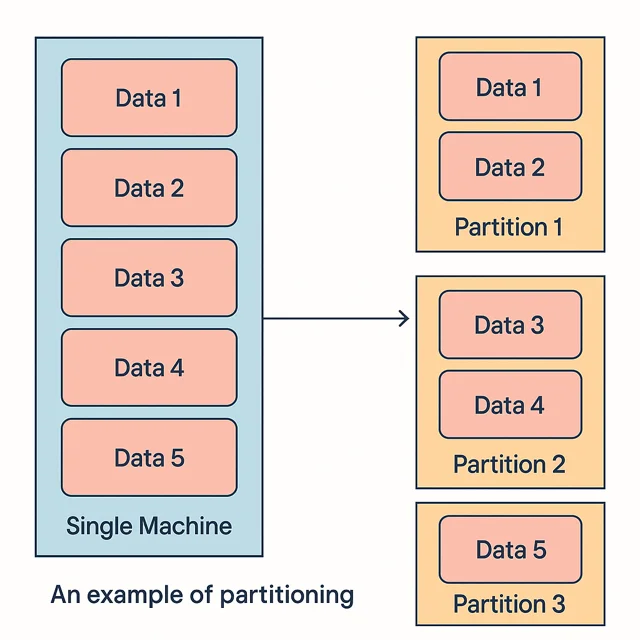
Every record in the database belongs to exactly one partition. Each partition acts as a database that can perform read and write operations on its own. We can either execute queries scoped to a single partition or distribute them across multiple partitions depending on the access pattern. For example, a query like: SELECT * FROM orders WHERE month(order_ts) = 10; targets only the October partition, enabling Iceberg to skip all irrelevant files entirely.

This process is critical for enhancing performance by reducing query scope (by scanning only relevant partitions instead of full datasets), enabling parallel processing (as different partitions can be read concurrently across multiple threads or nodes), and lowering storage costs (by avoiding redundant data duplication and minimizing the amount of data scanned during queries).

As data volumes continue to grow exponentially (to TBs)—driven by increased ingestion rates and analytics demands—the need for robust, flexible, and dynamically managed partitioning strategies has never been more acute.

Horizontal vs. Vertical Partitioning – Partitioning can be horizontal (splitting rows) or vertical (splitting columns). In horizontal partitioning, entire rows are separated into different tables or file sets based on some criteria, whereas vertical partitioning stores different columns in separate tables (often used to isolate cold infrequently-used columns).

This blog focuses on horizontal partitioning (splitting rows), as it’s the common approach for scaling large tables in databases and data lakes.

Common Partitioning Strategies: The most widely used horizontal partitioning strategies are:

• Range Partitioning: Each partition covers a continuous range of values for a partition key (such as dates or numeric IDs). For example, a sales table might be partitioned by date range, with one partition per year or month. Queries can then target a specific range (e.g. sales in 2023) and skip other partitions entirely.

• List Partitioning: Each partition is defined by an explicit list of values. For example, a table of customers could be partitioned by region or country, with one partition for “USA”, one for “EU”, etc. Data with a partition key matching one of the list values goes into the corresponding partition.

• Hash Partitioning: A hash function on a key (like user ID) determines the partition. This distributes rows evenly (pseudo-randomly) across partitions. Hash partitioning is useful when ranges or lists aren’t obvious, but you want to balance load. However, it’s considered the least useful strategy in many cases since it doesn’t group similar values – it’s mainly used to break up very large tables for manageability. For instance, hashing might split a 2TB table into 10 roughly equal 200GB partitions just to make vacuuming or maintenance faster.

• Composite Partitioning: Combining two or more methods, e.g. first partition by range, then within each range partition by list. This can handle complex data distributions. For example, partition a table by year (range), and within each year partition by region (list). Composite schemes offer flexibility but can be more complex to maintain.

Why Partitioning Matters

Why Partition? – The biggest benefit is query performance. Partitioning lets a query skip large chunks of data that are irrelevant. For example, if customers 0–1000 are in one partition and 1001–2000 in another, a query for customer ID 50 only needs to scan the first partition.

This partition pruning reduces I/O and speeds up the query. Partitioning also helps maintenance: each partition is smaller, making tasks like index rebuilds, backups, or deletes of old data (dropping a whole partition) more efficient. Partitioning can aid scalability by distributing data across disks or nodes, and can even improve availability by isolating failures to a subset of data. For instance, placing partitions on different nodes so one node’s failure only affects its partition.

These are the advantages of partitioning a database:

• Support for large datasets: The data is distributed across multiple machines beyond what a single machine can handle, thereby supporting large dataset use cases.
• Support for high throughput: Distributing data across multiple machines implies read and write queries can be independently handled by individual partitions. As a result, the database as a whole can support a larger throughput than what a single machine can handle.

Limitations of Traditional Partitioning: Classic partitioning isn’t a silver bullet. If not designed well, it can hurt performance – e.g. partitioning on a high-cardinality column (like a unique ID) creates many tiny partitions, causing overhead to manage and query them. Some strategies like hash make it hard to do targeted queries, since data is essentially randomly distributed.

In such cases, most queries end up scanning all partitions (defeating the purpose of partitioning). Additionally, older systems required a lot of manual setup and constraints: adding new partitions periodically, ensuring queries include partition filters, etc. There’s also a maintenance cost – each partition might need its own index or statistics, and too many partitions can overwhelm the query planner or metadata store.

Motivation for Evolving Partitioning Strategies
Traditional partitioning techniques, while effective in smaller environments, struggle under the weight of modern data volumes. The need for automated schema evolution, dynamic partition discovery, and reduced administrative overhead has spurred the development of advanced systems such as Apache Iceberg that decouple logical partitioning from physical storage structures.

Before delving into modern advancements, it is essential to appreciate how traditional systems, particularly Apache Hive, managed data partitioning.

Explicit (Folder-Based) Partitioning
In traditional databases, partitioning was most often implemented using an explicit, folder-based approach. Partition columns were mapped directly to physical directory structures on distributed file systems. This manual alignment meant that partitions had to be explicitly created, managed, and maintained through metadata updates and directory manipulation. While effective for smaller datasets, this approach incurs several limitations as datasets grow in size and complexity.

Challenges with Hive's Traditional Partition Management

Apache Hive pioneered the use of explicit partitioning in data lakes. By relying on manually defined partition columns and physical directory hierarchies, Hive allowed users to define clear segmentation of data. However, this strategy presented several inherent challenges:

• Manual Management: Partitions had to be manually created and maintained. As data evolved, the overhead of managing new partitions increased substantially.
• Inflexibility: Static partitioning schemes did not handle schema evolution systematically. Changing business requirements often demanded refactoring of the underlying storage layout.
• Query Performance Bottlenecks: Especially in cloud environments, overhead from file listing operations and partition pruning can degrade performance, particularly when the number of partitions becomes extremely high.

These issues catalyzed the movement toward more dynamic, metadata-driven solutions. Before we discuss these solutions, let us dig deeper into how partitioning works with Apache Hive.

Deep Dive into Apache Hive Partitioning

Mechanics of Hive Partitioning

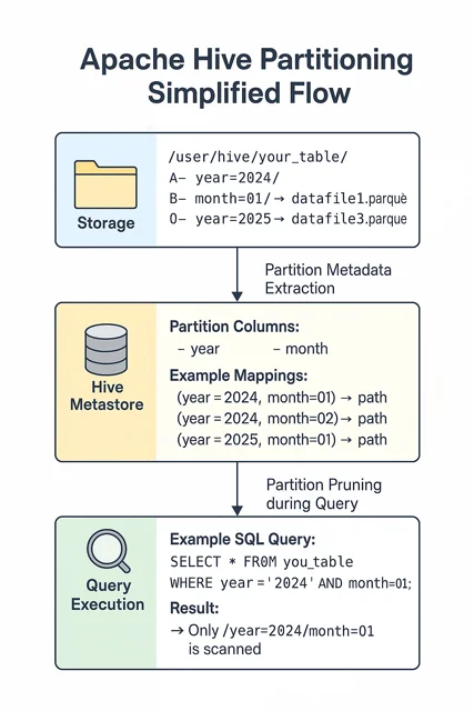
In Apache Hive, partitioning is achieved through the definition of explicit partition columns that correlate with physical directory paths in storage. The metadata stored in Hive’s metastore directly reflects this structure, meaning that query performance depends heavily on how well these partitions are maintained and pruned at query time.

Common Challenges and Bottlenecks

The traditional Hive approach often encounters several pain points:

• High File Listing Overhead: Especially in cloud storage environments (e.g., AWS S3), traversing large directory structures can become a performance bottleneck.
• Manual Schema Modifications: Schema changes and partition evolutions require manual updates across both the physical layout and the metadata, increasing the risk of error.
• Static Partitioning Strategies: Changing data patterns—such as variations in ingestion volume or dynamic schema evolution—are not easily accommodated without significant re-engineering.

For example, organizations often begin with a simple partitioning strategy, organizing their sales data by year and month, such as /sales/year=2024/month=04/. While effective under stable ingestion volumes — around 100,000 records per month — static partitions quickly become a bottleneck when volumes spike unexpectedly. A surge to 50 million records for April 2024 would overwhelm the monthly partition, leading to degraded query performance. Although day-level partitioning would better distribute the load, static designs lack the flexibility to adapt easily. Addressing this requires repartitioning existing data, refactoring ingestion pipelines, and rewriting queries, resulting in significant operational overhead and engineering effort.

These challenges set the stage for the introduction of more sophisticated partitioning techniques that emphasize automation and metadata abstraction, as seen in Apache Iceberg.

Apache Iceberg’s Innovative Partitioning Approach

Apache Iceberg represents a radical departure from traditional partitioning. Its focus on decoupling logical partitioning from physical layout has enabled several advances in how data lakes manage, evolve, and query datasets.

Hidden or Metadata-Driven Partitioning

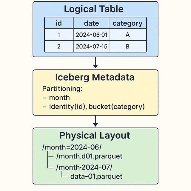
Iceberg introduces the concept of "hidden" partitions, where the partitioning information is maintained in the metadata layer rather than relying on folder structure. This metadata-driven approach provides several key benefits:

• Transparent Partition Management: Since partition information is embedded within the table metadata, end-users and query engines do not have to manage physical directories manually.
• Partition Evolutions: Iceberg supports automatic partition evolution, allowing the system to adapt partitioning schemes based on observed query patterns and evolving data distributions. Features like partition transforms enable on-the-fly modification of partition keys without the need for data reorganization.
• Decoupling from File Structure: By eliminating the strict dependency on folder hierarchies, Iceberg significantly reduces the performance overhead associated with file system operations and enables smooth schema evolution.

Support for Schema Evolution and Time Travel

Beyond partitioning, Iceberg also offers robust schema evolution capabilities. Alterations—adding or renaming columns, or even safe type promotions—are managed in a way that retains backward compatibility. Each change generates a new metadata snapshot (metadata.json), allowing for features such as time travel and versioned queries. This capability directly addresses the challenge of maintaining compatibility during a significant data transformation, ensuring that legacy queries continue to function with updated data models.

Partitioning in Apache Hive vs. Apache Iceberg

Partitioning behaves differently across database systems. Let’s compare how Apache Hive (a SQL-on-Hadoop engine), and Apache Iceberg (a modern table format for data lakes) approach partitioning.

Apache Hive’s Folder-Based Partitioning

Apache Hive, a SQL engine for Hadoop, uses a very explicit partitioning approach tied to the file system. When you partition a Hive table, each partition corresponds to a directory in HDFS containing the data files for that partition. The partition columns become part of the table’s metadata and also part of the file path. For example, if we partition a Hive table by a country field and a year field, Hive will organize files like:

/warehouse/my_table/country=US/year=2023/part-00001.parquet  
/warehouse/my_table/country=US/year=2024/part-00002.parquet  
/warehouse/my_table/country=IN/year=2023/part-00003.parquet  
... etc.

Each country=.../year=... subfolder holds the rows matching that partition combination. This is often called Hive-style partitioning. Querying the table with a filter on the partition columns (e.g. WHERE country='US' AND year=2023) will cause Hive (or other engines like Spark, Presto, Athena) to read only the files in that folder, skipping others – this is partition pruning by directory path.

To illustrate, let’s create a simple partitioned table in Hive and load some data:

-- 1. Create a partitioned Hive table  

CREATE TABLE logs (  
  level STRING,  
  message STRING,  
  event_time TIMESTAMP  
)  
PARTITIONED BY (event_date STRING)  -- partition key (typically a date or category)  
STORED AS PARQUET;

-- 2. Insert data into specific partitions (static partitioning)  

INSERT INTO logs PARTITION (event_date='2023-10-01')  
  VALUES ('INFO', 'Job started', '2023-10-01 09:00:00'),  
         ('ERROR','Job failed',  '2023-10-01 09:05:00');  
INSERT INTO logs PARTITION (event_date='2023-10-02')  
  VALUES ('INFO', 'Job started','2023-10-02 09:00:00');

In the above example, we explicitly insert data into two partitions: event_date=2023-10-01 and event_date=2023-10-02.

Physically, Hive will create folders .../logs/event_date=2023-10-01/ and .../logs/event_date=2023-10-02/ containing the respective data files.

If we run a query SELECT * FROM logs WHERE event_date='2023-10-01', Hive will read only the files in the event_date=2023-10-01 folder and not touch other dates.

Hive supports static partitioning (as above, where you specify the partition value on insert) and dynamic partitioning, where the partition value is determined at runtime from data.

For dynamic partitioning, you might insert from another table and let Hive split the output into partitions based on a column’s value. This requires enabling some settings (like hive.exec.dynamic.partition=true) and often a INSERT ... SELECT query that selects the partition key as a column.

One big characteristic of Hive partitioning is that it’s explicit – the partition columns are part of the table definition and need to be handled in queries. You usually include the partition column in your WHERE clause to benefit from partition pruning; otherwise, Hive will scan all partitions.

Another challenge is that Hive doesn’t inherently validate partition values against data – it’s possible to have data files in the wrong partition folder (say, a file in event_date=2023-10-01 folder actually containing some rows from 2023-10-02) if you’re not careful. The burden is on the user/ETL process to correctly assign partitions.

Changing a partitioning scheme in Hive later can be painful – it may involve creating a new table with a new partitioning and reloading or moving data.

Despite these drawbacks, Hive’s approach was straightforward and widely adopted for big data. It integrates with tools like Apache Spark, Presto, and AWS Athena which all understand Hive-style partitioned folders.

The explicit partition directories make it easy to add or drop partitions by adding folders, and Hive’s metastore keeps track of available partitions. However, as data scale grew (and the number of partitions grew), the Hive metastore could become a bottleneck, and the rigidness of explicit partition columns led to the evolution of new approaches like Iceberg.

Apache Iceberg’s Metadata-Driven Partitioning

Apache Iceberg is a next-generation table format that handles partitioning quite differently. Iceberg introduces hidden partitioning, meaning the details of partitioning are abstracted away from the user – you don’t need to manually manage partition columns in your data or queries. Instead, Iceberg uses a metadata layer (manifest files, etc.) to track which data files belong to which partitions, and it automatically applies partition pruning based on query filters.

When you create an Iceberg table, you still specify a partitioning strategy, but it’s done in a declarative way. For example, in a Spark SQL or Iceberg SQL environment, you might do:

-- Creating an Iceberg table with partition transforms  
CREATE TABLE sales_data (  
  sale_id BIGINT,  
  amount  DECIMAL(10,2),  
  sale_ts TIMESTAMP,  
  region  STRING  
)  
USING iceberg  
PARTITIONED BY (days(sale_ts), region);

This defines an Iceberg table partitioned by day of sale timestamp and region. Unlike Hive, we don’t have to add an extra sale_date column or manually manage region-based directories — Iceberg automatically handles partitioning based on existing columns. Also, the query interface doesn’t change; we would query this table by sale_ts or region normally, and Iceberg will ensure it reads only the needed partitions.

Iceberg partitioning supports transform functions on values, as shown above (days(sale_ts)). Other supported transforms include year(), month(), hour(), bucket(N, column) for hashing into N buckets, and truncate(length, column) for prefix truncation. This means you can partition by a year or month of a timestamp, or by a hash bucket, without creating separate columns – Iceberg handles computing the partition values. These are essentially the partition spec for the table.

Under the hood, Iceberg does not rely on directory names for partition pruning (though it may still organize files in folders). Instead, it maintains metadata files (manifests) that list all data files and their partition values. When a query with a filter comes in, Iceberg’s API will read the metadata to quickly find which files satisfy the filter (e.g., which files have sale_ts in 2023 and region = 'EU').

This means no expensive directory listing at query time, and it also means users don’t need to include partition columns in queries – filtering on the original column is enough. For example, a query SELECT SUM(amount) FROM sales_data WHERE sale_ts >= '2023-10-01' AND sale_ts < '2023-11-01' AND region='EU' will automatically be pruned to only files in the October 2023 + EU partition, even though the query never mentioned “partition” or a separate date column.

Another advantage is evolution: Iceberg allows changing the partition scheme without rewriting all data. You could repartition new data differently (a feature called partition evolution), and Iceberg can query both old and new partitions seamlessly. Also, Iceberg validates partition values at write time (since it’s doing the computation), preventing issues like data in wrong partitions.

A quick over of Iceberg’s approach to partitioning:

• No need to manage partition columns in data loading or querying – the framework takes care of it.
• Rich partition transforms out of the box (date/time, bucket, truncate).
• Metadata-driven – queries consult a centralized metadata (often a Metastore or catalog service) to find relevant data files, rather than hitting the filesystem for each partition. This is faster and scales to many more partitions.
• ACID compliance and time travel – as a bonus, Iceberg tables support atomic changes and snapshot isolation, so adding or removing data files (even in different partitions) is transactional and consistent.

Comparative Analysis of Partitioning Approaches

Let’s compare how Hive, and Iceberg partitioning stack up in real-world scenarios, focusing on performance, manageability, and use cases.

Performance and Query Speed

All partitioning methods aim to improve query speed by reading less data. In traditional databases like PostgreSQL or in Hive, if a query can use the partition key in a filter, it will only scan that partition instead of the whole table – potentially speeding up queries by orders of magnitude if the data is large.

For example, Amazon Athena (which queries Hive-style data on S3) only reads the partitions needed, significantly cutting scan time and cost for partitioned data. However, Hive partitioning has some overhead: each query may need to communicate with the Hive metastore to fetch partition locations, and if you have thousands of partitions, planning the query can become slower.

Iceberg’s design generally yields equal or better performance for partitioned queries. Because Iceberg keeps an index of files (in manifests), it can quickly prune out not just partitions but individual files that don’t match a filter. This can outperform Hive in scenarios with many small partitions.

In one financial use-case, adopting Iceberg showed query performance improvements up to 52% faster compared to querying the same data in a “vanilla” Hive/Parquet layout (Build a high-performance quant research platform with Apache Iceberg | AWS Big Data Blog). This is partly due to Iceberg’s ability to avoid full directory scans and skip metadata overhead, and also thanks to additional features like data file pruning (skipping irrelevant files based on statistics).

Storage Efficiency: Partitioning can have side effects on storage. In Hive, each partition often results in multiple small files (especially if data ingestion is frequent and not consolidated). Lots of small files are inefficient on HDFS/S3 because of high overhead per file. A gaming company with massive log data (Tencent Games) found that their old Hive-based pipeline required many pre-aggregations (materialized summaries per partition) to get decent performance. By unifying data on Iceberg and using its features, they eliminated those extra data copies and reduced storage costs by 15x (Apache Iceberg | CelerData).

Iceberg helps here by enabling on-the-fly aggregation (with query engines reading base detail data) and by offering table-level compaction to merge small files.

One thing to consider is metadata storage.

Hive keeps partition info in its metastore (or Glue catalog) – if you have a partition for every day over 10 years, that’s 3,650 entries plus potentially subpartitions, etc. Very fine-grained partitions (e.g. per hour or per user) can bloat the Hive metastore and even exceed its capacity. Iceberg’s metadata (manifest files and a single table entry in the catalog) is typically more compact and scales to a huge number of partitions because it doesn’t rely on one metastore row per partition.

Imagine you want to partition clickstream data by hour over 3 years:

• Hive:
  24 hours/day × 365 days/year × 3 years = 26,280 partitions
  → 26,280 rows in the metastore.
  → Every query needs to scan partition metadata for thousands of entries.

• Iceberg:
  Just one table entry in the catalog.
  All the partitioning by hour is handled via manifests.
  Query reads only relevant manifests efficiently — no explosion in the catalog.

This makes Iceberg more scalable in terms of number of partitions – you could partition by hour or have thousands of bucket partitions without crashing your catalog service.

Ease of Management

From a developer/operator perspective, Iceberg is the clear winner in ease of partition management. You don’t have to manually add partitions or repair tables – when you insert data, Iceberg writes new files and updates metadata in one transaction. In Hive, you often had to run ALTER TABLE ADD PARTITION or MSCK REPAIR TABLE to tell the metastore about newly added partition folders (unless you used Hive’s insertion which does it for you). Forgetting to do this would result in data not found by queries.

Also, with Hive you had to always remember to include partition filters in your queries (or else suffer a full scan), whereas Iceberg spares you that concern – you just query naturally by any filter, and if it happens to align with a partition, great, it will prune it for you automatically.

Iceberg shines in flexibility. Need to repartition the table? Iceberg allows adding a new partition spec. Need to roll back a change or query as of a previous data load? Iceberg supports time travel by snapshots. These go beyond partitioning but are related to how it manages data at a higher level. Another convenience: migrating a table’s storage format (say Parquet to ORC) or compacting files is straightforward with Iceberg; with Hive you’d have to run a possibly expensive ETL job to rewrite the data.

Scalability and Use Cases

In modern big data scenarios:

• Hive partitioning was designed for huge scale on HDFS – multi-terabyte tables. It’s batch-oriented; good for nightly aggregations or historical analysis where you can afford a MapReduce or Spark job scanning partitions. Many firms (ad-tech, telecom, etc.) used Hive to store logs partitioned by date. The limitation is the query engines (MapReduce/Tez) were not interactive, and the maintenance could get cumbersome with thousands of partitions.
• Iceberg is built for lakehouse environments – large-scale analytics with multiple engines (Spark, Trino/Presto, Flink, etc.) and is cloud-friendly. Fintech companies are adopting Iceberg for things like transaction data lakes or market data: query engines can do interactive analytics on petabytes of data partitioned by date or asset, and they benefit from Iceberg’s reliable schema and partition management. In the gaming industry, as mentioned, Iceberg helps unify real-time and batch data.

A real example: Tencent’s gaming analytics moved from a lambda architecture (separate real-time DB and offline Hive store) to Iceberg, allowing them to query fresh and historical data in one place and simplifying their pipeline (no separate pre-aggregation store) (Apache Iceberg | CelerData). This illustrates better scalability not just in data size, but in data architecture simplicity.

Partitioning is indispensable for large datasets, but the technology you use dictates how much work it is to get right. Hive showed how partitioning can scale to big data, but at the cost of more manual management and less flexibility. Iceberg and similar modern table formats (Delta Lake, Hudi) build on those lessons to give us the best of both worlds: the scale of data lakes with the manageability of databases. Partitioning in Iceberg is practically set-and-forget, allowing us to focus on using the data rather than babysitting partitions.

Comparative Analysis: Hive vs. Iceberg

Side-by-side analysis of Apache Hive’s traditional partitioning and Apache Iceberg’s modern approach, focusing on cloud-native environments.

Feature / Metric	Apache Hive Partitioning	Apache Iceberg Partitioning
Partition Management	Manual, explicit, folder-based	Metadata-driven (hidden partitions)
Schema Evolution	Challenging, manual interventions required	Automated, transparent with time travel support
Query Performance (Cloud)	Degradation with high file list operations	Faster due to reduced file I/O and metadata layering
Ease of Integration	On-prem oriented, less flexible	Cloud-native integrations (AWS Athena, Spark, Dremio)
Migration Complexity	Manual partition-specific migrations	In-place vs. shadow migrations with blue/green deployment

Next, let’s put some of this into practice with a quick implementation guide using Docker.

Implementation Guide with Docker: Hive and Iceberg in Action

For a hands-on understanding, it’s useful to try creating and querying partitioned tables yourself. In this guide, we'll create two tables — one in Hive and one in Iceberg — populate them with datasets, and observe how partitioning impacts query performance and behavior.

Environment Setup: We will use the official Apache Hive Docker image, which conveniently comes with Iceberg support. This single container will run Hive Metastore and HiveServer2, and includes the Iceberg runtime libraries so that Hive can create Iceberg tables. Ensure you have Docker installed, then run:

# Pull and start Hive 4.0 (which we use for Iceberg compatibility)

export HIVE_VERSION=4.0.0  
docker run -d -p 10000:10000 -p 10002:10002 \  
    --env SERVICE_NAME=hiveserver2 --name hive4 \  
    apache/hive:${HIVE_VERSION}

This launches a Hive server container listening on port 10000 (the JDBC interface) (Hive and Iceberg Quickstart - Apache Iceberg™). It uses an embedded Derby database for the Hive Metastore by default, which is fine for our demo. The Hive Metastore will act as the catalog for Iceberg tables as well, storing table metadata and schemas.

Next, connect to Hive using Beeline (the Hive shell):

docker exec -it hive4 beeline -u "jdbc:hive2://localhost:10000/default"

This drops you into a SQL prompt. Now we can execute Hive SQL commands.

Create and use a demo database

CREATE DATABASE demo;  
USE demo;

Create a Hive partitioned table

Let’s make a traditional Hive-managed partitioned table and insert data.

CREATE TABLE hive_orders (  
  order_id INT,  
  product  STRING,  
  price    DOUBLE  
)  
PARTITIONED BY (order_date STRING)  
STORED AS PARQUET;

Next, populate the table with approximately 30,000 rows across three partitions:

CREATE TABLE numbers (n INT);

INSERT INTO numbers VALUES   
(0),(1),(2),(3),(4),(5),(6),(7),(8),(9),  
(10),(11),(12),(13),(14),(15),(16),(17),(18),(19),  
(20),(21),(22),(23),(24),(25),(26),(27),(28),(29),  
(30),(31),(32),(33),(34),(35),(36),(37),(38),(39),  
(40),(41),(42),(43),(44),(45),(46),(47),(48),(49),  
(50),(51),(52),(53),(54),(55),(56),(57),(58),(59),  
(60),(61),(62),(63),(64),(65),(66),(67),(68),(69),  
(70),(71),(72),(73),(74),(75),(76),(77),(78),(79),  
(80),(81),(82),(83),(84),(85),(86),(87),(88),(89),  
(90),(91),(92),(93),(94),(95),(96),(97),(98),(99);

For each partition:

INSERT INTO hive_orders PARTITION (order_date='2022-10-01')  
SELECT  
  n1.n * 100 + n2.n AS order_id,  
  CONCAT('Product_', CAST(n1.n * 100 + n2.n AS STRING)) AS product,  
  rand() * 100 AS price  
FROM numbers n1  
CROSS JOIN numbers n2;

INSERT INTO hive_orders PARTITION (order_date='2022-11-01')  
SELECT  
  n1.n * 100 + n2.n AS order_id,  
  CONCAT('Product_', CAST(n1.n * 100 + n2.n AS STRING)) AS product,  
  rand() * 100 AS price  
FROM numbers n1  
CROSS JOIN numbers n2;

INSERT INTO hive_orders PARTITION (order_date='2022-12-01')  
SELECT  
  n1.n * 100 + n2.n AS order_id,  
  CONCAT('Product_', CAST(n1.n * 100 + n2.n AS STRING)) AS product,  
  rand() * 100 AS price  
FROM numbers n1  
CROSS JOIN numbers n2;

Now, the table has ~30,000 rows partitioned across three different order_date values.

You can verify the partitions:

SHOW PARTITIONS hive_orders;

Expected output:

+------------------------+  
|       partition        |  
+------------------------+  
| order_date=2022-10-01  |  
| order_date=2022-11-01  |  
| order_date=2022-12-01  |  
+------------------------+  
3 rows selected (0.065 seconds)

Querying Hive Correctly to Take Advantage of Partitioning

Run this query:

SELECT * FROM hive_orders  
WHERE date_format(order_date, 'yyyy-MM-dd') BETWEEN '2022-10-01' AND '2022-12-31';

-Output  
30,000 rows selected (0.624 seconds)

Although the intent was to select order between '2022-10-01' and '2022-12-31' Hive cannot recognize the partition pruning opportunity. As a result, all partitions are scanned unnecessarily, even if only a subset of the data is needed.

Why This Happens

In Hive's directory-based partitioning:

• Partitions are mapped to physical directories (order_date=...).

• The Metastore can only prune partitions if the query directly references the partition column without transformations.

• Functions applied to partition columns break the pruning optimization.

Create an Iceberg Partitioned Table

Now for comparison, let’s create an Iceberg table in the same Hive environment. Since we have Hive 4 with Iceberg, the syntax is a bit different – we use STORED BY ICEBERG to denote an Iceberg table. We’ll also use Iceberg’s partition transforms.

-- Create an Iceberg table partitioned by year of a timestamp and by category

CREATE TABLE iceberg_orders (  
  order_id INT,  
  product  STRING,  
  price    DOUBLE,  
  ts       TIMESTAMP,  -- order timestamp  
  category STRING  
)  
PARTITIONED BY SPEC (  
  MONTH(ts)             -- partition by month extracted from ts  
)  
STORED BY ICEBERG;

In the above, PARTITIONED BY SPEC (...) is Iceberg’s way of specifying partition transforms in Hive (Creating an Iceberg partitioned table). We partition iceberg_orders by year and by month. Iceberg will handle the logic of mapping each row to the correct year and month behind the scenes.

Load the Iceberg table with approximately 30,000 rows:

Expand the numbers table:  
INSERT INTO numbers VALUES   
(100),(101),(102),(103),(104),(105),(106),(107),(108),(109),  
(110),(111),(112),(113),(114),(115),(116),(117),(118),(119),  
(120),(121),(122),(123),(124),(125),(126),(127),(128),(129),  
(130),(131),(132),(133),(134),(135),(136),(137),(138),(139),  
(140),(141),(142),(143),(144),(145),(146),(147),(148),(149),  
(150),(151),(152),(153),(154),(155),(156),(157),(158),(159),  
(160),(161),(162),(163),(164),(165),(166),(167),(168),(169),  
(170),(171),(172),(173),(174),(175),(176),(177),(178),(179),  
(180),(181),(182),(183),(184),(185),(186),(187),(188),(189),  
(190),(191),(192),(193),(194),(195),(196),(197),(198),(199),  
(200),(201),(202),(203),(204),(205),(206),(207),(208),(209),  
(210),(211),(212),(213),(214),(215),(216),(217),(218),(219),  
(220),(221),(222),(223),(224),(225),(226),(227),(228),(229),  
(230),(231),(232),(233),(234),(235),(236),(237),(238),(239),  
(240),(241),(242),(243),(244),(245),(246),(247),(248),(249),  
(250),(251),(252),(253),(254),(255),(256),(257),(258),(259),  
(260),(261),(262),(263),(264),(265),(266),(267),(268),(269),  
(270),(271),(272),(273),(274),(275),(276),(277),(278),(279),  
(280),(281),(282),(283),(284),(285),(286),(287),(288),(289),  
(290),(291),(292),(293),(294),(295),(296),(297),(298),(299);

INSERT INTO iceberg_orders  
SELECT  
  n1.n * 100 + n2.n AS order_id,  
  CONCAT('Product_', CAST(n1.n * 100 + n2.n AS STRING)) AS product,  
  rand() * 100 AS price,  
  from_unixtime(  
    unix_timestamp('2022-10-01', 'yyyy-MM-dd') +  
    (n1.n * 100 + n2.n) % 90 * 86400  
  ) AS ts,  
  CASE WHEN (n1.n * 100 + n2.n) % 2 = 0 THEN 'electronics' ELSE 'furniture' END AS category  
FROM numbers n1  
CROSS JOIN numbers n2  
WHERE n1.n < 300 AND n2.n < 100  
ORDER BY month(  
  from_unixtime(  
    unix_timestamp('2022-10-01', 'yyyy-MM-dd') +  
    (n1.n * 100 + n2.n) % 90 * 86400  
  )  
);

This data spans over 90 days, distributed across October, November, and December 2022.

Querying Iceberg Tables

In Iceberg, querying is natural and partition pruning happens automatically.

Query without worrying about partitions:

SELECT * FROM iceberg_orders  
WHERE month(ts) = 10;

-output  
10,353 rows selected (0.191 seconds)

Iceberg will:

• Analyze the query predicate,

• Push the filter down based on MONTH(ts) partitioning,

• Automatically skip non-matching partitions.

A full table scan would have taken 0.461 seconds.

There is no need to manually filter by month columns. Iceberg leverages hidden partitioning metadata for optimization.

Explore Metadata

You can use DESCRIBE FORMATTED database.table_name; in Hive to see details about the tables.

DESCRIBE FORMATTED demo.hive_orders;  
DESCRIBE FORMATTED demo.iceberg_orders;

Notice how:

• Hive shows order_date as a physical partition column.

• Iceberg shows partition specs using transformations like YEAR(ts) and BUCKET(category).

If you dive into the filesystem (docker exec -it hive4 hadoop fs -ls /user/hive/warehouse/demo.db/), you'll see Hive’s folder structure — but Iceberg might organize data differently (or even flatten it), because folder names don't matter for Iceberg.

The key difference is, Iceberg’s query engine doesn’t rely on those folders.

This simple exercise shows that from the usage perspective, querying an Iceberg table is just like a normal SQL table (no need to mention partitions in the query), whereas the Hive table requires you to be partition-aware. In terms of SQL, they feel similar when inserting (Hive needed PARTITION(...) clause on insert, Iceberg did not).

Maintenance-wise, if you had more data to add for a new date in Hive, you’d either insert with the correct partition or add a partition then load data. In Iceberg, you just insert data and it will automatically add new partition entries as needed.

Cleanup
When done, you can exit Beeline (!quit) and stop the Docker container (docker stop hive4 && docker rm hive4). This was a minimal setup. In a real scenario, you might use a separate metastore service and engines like Spark or Trino to interact with Iceberg tables. But the concepts would remain the same.

Conclusion

The shift from traditional Hive partitioning to Apache Iceberg’s metadata-driven approach marks a major step forward in how modern data lakes are built. By separating how data is logically partitioned from how it's physically stored, Iceberg overcomes many of the pain points of folder-based partitioning—like rigid directory structures and complex schema updates.

Features like automatic partition management, seamless schema evolution, and tight cloud integration lead to real improvements in query speed, cost savings, and day-to-day operations. Companies are seeing these benefits firsthand, reporting significant gains in performance and efficiency.

Even when it comes to migration, Iceberg supports practical, low-risk strategies like in-place upgrades or shadow deployments with blue/green rollouts, making the move from Hive to Iceberg more approachable for large teams.

Apache Iceberg brings a more modern, flexible, and scalable foundation for managing data in today’s cloud-native environments.

Note: The research and benchmarks discussed in this report are based on both documented case studies and independent benchmarks from leading vendors and technical communities. While speculative predictions suggest further significant performance improvements as additional tools and optimizations are integrated, enterprises should evaluate strategies based on their unique workloads and growth trajectories.

OLake

Achieve 5x speed data replication to Lakehouse format with OLake, our open source platform for efficient, quick and scalable big data ingestion for real-time analytics.

Schedule a meetSignupExplore OLake GitHub

Contact us at hello@olake.io